2.1.2.1 Autocorrelation and Partial Autocorrelation (ACF & PACF)

1 Summary
2 Tutorial
- 2.1 ACF & PACF
3 Algorithm
- 3.1 Autocorrelation
- 3.2 Partial Autocorrelation
4 Reference

Summary

This ACF(Autocorrelation function) & PACF( Partial Autocorrelation function) tool is supported in the Time Series Analysis App. It is used to compute and plot the autocorrelations and the partial autocorrelations of a series.

Tutorial

This tutorial uses App’s built-in sample project. To open this sample OPJU file:

Right click the Time Series Analysis App icon in the Apps Gallery and choose Show Samples Folder.
A folder will open. Drag-and-drop the project file TSA Sample.opju into Origin.

ACF & PACF

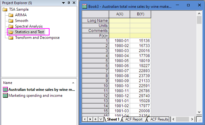
Expand Project Explorer docked on the left. Select folder Statistics and Test . The Book3 contains data about Australian total wine sales by wine makers in bottles.
Highlight Column A and B, and then click the Time Series Analysis App icon in the Apps Gallery.
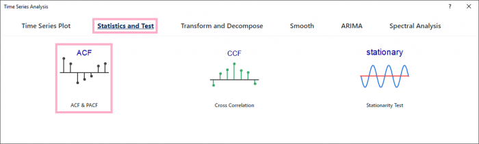
In the dialog, select Statistics and Test and ACF & PACF tool.
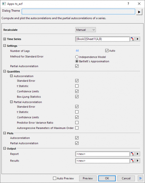
Use the default dialog setting, click the OK button.
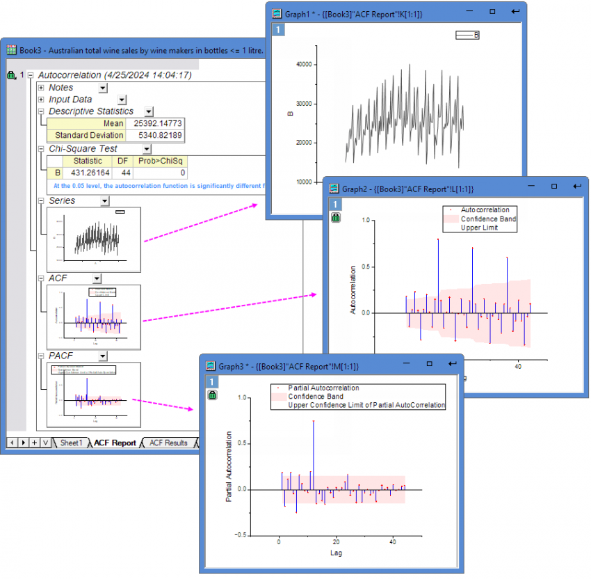
Then you will get the report with Series, ACF and PACF three graphs.

Algorithm

Autocorrelation

Autocorrelation calculates the correlation between a time series and the time series with lags. It can be used to determine which terms to be included in ARIMA model.

This app calls nag_tsa_auto_corr (g13abc) function [1] to calculate autocorrelation.

For a time series $x_i$ , i=1, 2, ... n, the coefficient of lag k is:

$r_k = \frac{ \displaystyle \sum_{i=1}^{n-k} (x_i - \bar{x}) (x_{i+k} - \bar{x})}{ \displaystyle \sum_{i=1}^n (x_i - \bar{x})^2 }$

where $\bar{x} = \frac { \sum_{i=1}^n x_i }{n}$ .

Default Maximum Number of Lags

$n_k = \begin{cases} n/4 \quad &\text{if } n \le 240 \\ 45 + \sqrt{n} \quad &\text{otherwise}\end{cases}$

Chi-squared Test

H₀: The autocorrelation function is identically zero.

$\chi^2 = n \displaystyle\sum_{k=1}^{n_k} r_k^2$

$\text{df} = n_k$

If P-value<0.05, the autocorrelation function is significantly different from zero.

Standard Error of Autocorrelation

1. Independent model

$s_k^2 = \frac{n - k}{ n (n + 2)}, k=1, 2, ..., n_k$

2. Bartlett model

$s_k^2 = \frac{1 + 2 \displaystyle\sum _{i=1}^{k - 1} r_i^2}{n}, i=1, 2, ... n_k$

t-value and Confidence Limits

$t_k = \frac{r_k}{s_k}$

Lower confidence limit at lag k:

$LCL_k = -2 s_k$

Upper confidence limit at lag k:

$UCL_k = 2 s_k$

Ljung-Box Test

H₀: First k autocorrelations are identically zero.

$Q_k = n (n+2) \displaystyle\sum_{i=1}^{k} \frac{r_i^2}{n-i}$

$\text{df}_k = k$

Use $\chi^2$ distribution to calculate the P-value.

If P-value<0.05, first k autocorrelations are significantly different from zero.

Partial Autocorrelation

Partial autocorrelation calculates the correlation between a time series and the time series with lags excluding the influence of intermediate lags. It can be used to determine terms to include in ARIMA model.

This app calls nag_tsa_auto_corr_part (g13acc) function [3] to calculate partial autocorrelation.

For a time series $x_i$ , i=1, 2, ... n, partial autocorrelation coefficients can be solved by a recursive method [4]:

$p_{l+1, l+1 } = ( r_{l+1} - p_{l, 1} r_l - p_{l, 2} r_{l-1} - ... - p_{1, l} r_1 )/ v_l$

$p_{l+1, j} = p_{l, j} - p_{l+1, l+1} p_{l, l+1-j}, \; j=1, 2, ..., l$

$v_{l+1} = v_l (1 - p_{l+1, l+1}) (1 + p_{l+1, l+1})$

where $l=1, 2,\, ...,\, n_k-1$ ,

$r_i, \, i=1, 2,\, ...,\, n_k$ is autocorrelation,

$v_i, \, i=1, 2,\, ...,\, n_k$ is the predictor error variance ratio,

$p_{i, i}, \, i=1, 2,\, ...\, n_k$ is partial autocorrelation values, and $p_{n_k, j}, \, j=1, 2,\, ...,\, n_k$ is the autoregressive parameters of maximum order.

It was initialized by setting $p_{1, 1} = r_1$ and $v_1 = 1 - r_1^2$ .

Standard Error of Partial Autocorrelation

$s_k = \frac{1}{\sqrt{n}}$

t-value and Confidence Limits

$t_k = p_{k, k} \cdot \sqrt{n}$

Lower confidence limit at lag k:

$LCL_k = -2 s_k$

Upper confidence limit at lag k:

$UCL_k = 2 s_k$

Reference

nag_tsa_auto_corr (g13abc)
George E. P. Box and Gwilym M. Jenkins (1976). Time Series Analysis: Forecasting and Control. (Revised Edition) Holden–Day
nag_tsa_auto_corr_part (g13acc)
J. Durbin (1960). The fitting of time series models. Rev. Inst. Internat. Stat. Vol.28, pp.233