4.2.2.6 User Defined Fitting Function

1 Summary
2 What You Will Learn
3 How to Create a Fitting Function and Use it to Perform Curve Fitting
- 3.1 Method 1: Using Simple Fit app
- 3.2 Method 2: Using Fitting Function Organizer and NLFit Tool
  - 3.2.1 Step 1: Create a Fitting Function Using Fitting Function Organizer
  - 3.2.2 Step 2:Carry Out Curve Fitting using NLFit Tool

Use Initial Formula to Better Guess Fitting Parameter Values from Data

Summary

Besides the 200+ built-in fitting functions, you can also create your own fitting functions in Origin. A number of Origin tools support fitting with your own functions, including:

Simple Fit App
Simple Fit App provides a much more convenient way to fit simple functions that can be expressed in the form y = f(x), you only need to type your formula or select an existing function, specify the initial values and then generate fitting reports immediately. You can learn how to use this App in this section.
Note: The Simple Fit app is pre-installed with Origin program, you can call it from the App Gallery with a graph window activated.
Qucik Fit Gadget
Quick Fit gadget is another easy way to do both linear and nonlinear fitting without open the Linear Fit or NLFit dialog which might look a little bit complicated but with many advanced controls. Start a fitting process with this gadget, you need first add your own function into the Function List.
NLFit tool.
NLFit tool is a powerful fitting wizard which allows you to define more complex fitting functions and control the fitting process in every possible way. For fitting user defined function in NLFit tool, you will need to create it in Fitting Function Builder first.

In this tutorial, we will mainly illustrate how to create a user-defined fitting function in Fitting Function Builder, carry out nonlinear curve fit with it and also show how to fix a parameter for curve fitting using NLFit tool.

Minimum Origin Version Required: Origin 2016 SR0

What You Will Learn

This tutorial will show you how to:

Create a user-defined fitting function
Carry out nonlinear curve fit with user-defined fitting function.

How to Create a Fitting Function and Use it to Perform Curve Fitting

The data we are going to fit is the file ConcentrationCurve.dat under the <Origin EXE Folder>\Samples\Curve Fitting\ path.

The fitting function to be created and used is shown below:

$y=A\exp(2.303kx-k_{m})\sqrt{2.303+\frac{C}{(x-C_{0})}}$

in which

$y$ is the dependent variable

$x$ is the independent variable

and $A, k_{m}, k, C, C_{0}$ are all fitting parameters.

Method 1: Using Simple Fit app

Create a new workbook.Click the button to import the ConcentrationCurve.dat file under <Origin EXE Folder>\Samples\Curve Fitting\ path.
Highlight column B and click the button to generate a scatter plot.
Click on Simple Fit icon from the Apps panel to open the Simple Fit app. Switch to Nonlinear tab, enter the equation in the y(x)= box. And then the parameter table will appear to let you enter the initial values for the parameters.
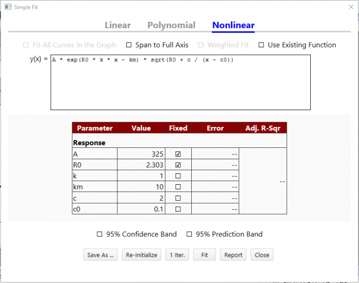
Once the equation has been entered and parameters have been initialed and fixed, click Fit button to fit the curve with the function you just defined. Of course, you can check the trend of fitting by clicking 1 Iter. button once by once.
You can click Save As... to save this function for further use. Click Close button to check the fitting results.

Method 2: Using Fitting Function Organizer and NLFit Tool

Step 1: Create a Fitting Function Using Fitting Function Organizer

In this section, we will show how to create a user defined fitting function in the Fitting Function Builder. But there is an alternative tool Fitting Function Organizer which also can be used to create user defined fitting functions(open it by selecting Tools: Fitting Function Organizer or pressing F9).

Launch Origin and choose Tools: Fitting Function Builder (or press F8) to open the Fitting Function Builder.
In the Goal page, select Create a New Function and click Next.
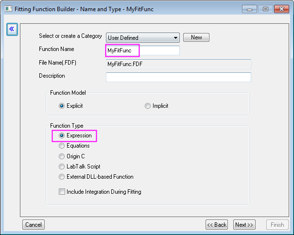
In the Name and Type page, change the setting as the following image and then click Next:
In the Variables and Parameters page, enter the variable and parameter names as the image below and then click Next:

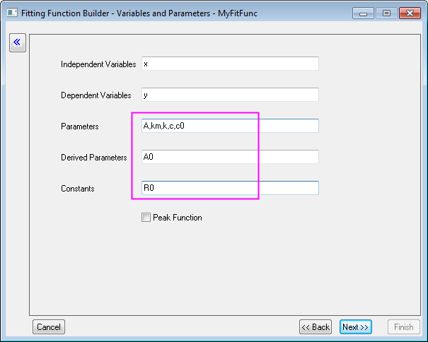
In the Parameters box, use comma (",") as delimiter.
In the Expression Function page, enter the equation below in Function Body:
```
A*exp(R0*k*x-km)*sqrt(R0+c/(x-c0))
```
Go to the Constant tab, set the value of R0 to 2.303.
Give estimated initial values to the parameters according to this particular data and function.

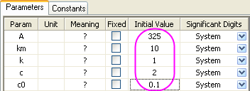
Note:You can also give different initial values each time before you actually carry out the fitting.
Can click the Evaluate button to quick check whether the function is valid(if it is valid, an actual value will be returned for y).
Note:If you used Origin C as Function Type at the beginning, you can also compile the function at this stage to check if there is any error, this is especially useful for brackets matching.
Click the Next button three times until it goes to Derived Parameters page.
In this page, we will define the derived parameter A0, enter its equation in the Derived Parameters Equations box:
```
A0=-A*exp(km)*1E-4
```
Click Finish to create this user defined fitting function. The .FDF file for it will be stored in the User Files Folder.

You can always modify the user defined fitting function later, either in the Fitting Function Builder(choose Edit a User-defined Function in Goal page), or in the Fitting Function Organizer.

Step 2:Carry Out Curve Fitting using NLFit Tool

Create a new workbook.Click the button to import the ConcentrationCurve.dat file under <Origin EXE Folder>\Samples\Curve Fitting\ path.
Highlight column B and click the button to generate a scatter plot.
Keep the graph activated, select Analysis:Fitting:Nonlinear Curve Fit to open the NLFit dialog.
In the Function Selection page, set Category as User Defined and then set Function as MyFitFunc(User).
Click the button to fit the data.
An error message returns in the Message tab of the lower panel, indicates the fit did not converge because of overparameterization.
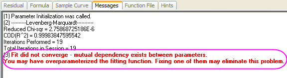
The parameters A and km have mutual dependence, so fixing either one will solve the problem. We will fix A this time.
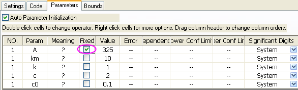
Go to the Parameters tab, click the to restore the initial value setting, check the Fixed box of parameter A:
Click the Fit button to carry out the fit.
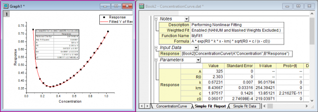
The fitted curve will be added to the original data plot,
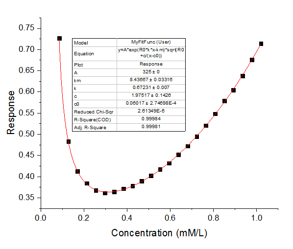
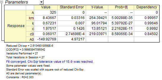
A report sheet will be generated as well, in which the fitted value of all parameters(including the derived parameter A0) are reported in the parameters table:

In the case of overparameterization, you can fix different parameters to get multiple fit results and then compare the fit models statistically by Analysis:Fitting:Compare Models tool.