4.2.2.2 Nonlinear Fitting with System Function

1 Summary
2 What you will learn
3 Steps

Summary

The NLFit dialog is an interactive tool which allows you to monitor the fitting procedure during the non-linear fitting process. This tutorial fits the Michaelis-Menten function, which is a basic model in Enzyme Kinetics, and shows you some basic features of the NLFit dialog. During the fitting, we will illustrate how to perform a Global Fit, which allows you to fit two datasets simultaneously and share some parameter values.

Minimum Origin Version Required: Origin 8.0 SR6

What you will learn

This tutorial will show you how to:

Import a single ASCII file.
Perform a global fit with shared parameters.
Select a fitting range and fit part of the data.
Use the Command Window to perform a simple calculation.

Steps

Import the file

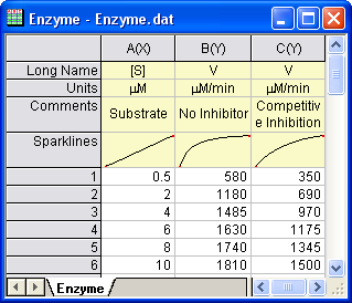
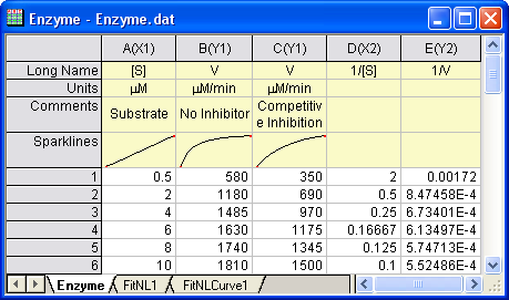
Open a new workbook. Select Help: Open Folder: Sample Folder... to open the "Samples" folder. In this folder, open the Curve Fitting subfolder and find the file Enzyme.dat. Drag-and-drop this file into the empty worksheet to import it.

Plotting the Data

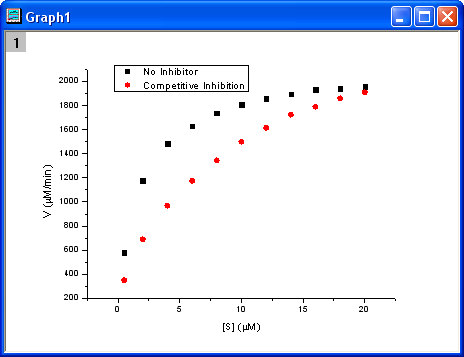
Select columns B and C and plot as a scatter plot by clicking the button.

Fitting with the Michaelis-Menten Function

The single-substrate Michaelis-Menten function is a basic model used in enzyme kinetics studies.

$v=\frac{V_{max}[S]}{K_m+[S]}$

The parameter $v$ is the reaction velocity, $[S]$ is the substrate concentration, $V_{max}$ is the maximal velocity, and $K_m$ represents the Michaelis constant. Parameters $V_{max}$ and $K_m$ are important enzyme properties and their values can be determined by fitting the M-M function to a $v$ vs. $[S]$ curve. While there is no M-M fitting function in Origin, we can use a more general model, the built-in Hill function to perform the fit:

$v=V_{max}\frac{x^n}{k^n+x^n}$

where $n$ is the cooperative sites. For a single-substrate model, we fix $n=1$ , thus simplifying the model so that it behaves like the M-M function.

There are two curves, one is the reaction without an Inhibitor and the other is the reaction with a Competitive Inhibitor. We will use the NLFit tool to fit these two curves simultaneously. Since for competitive inhibition reactions, the maximum velocity is the same as with no inhibition, we can share the $V_{max}$ value during the fitting procedure and perform a Global Fit.

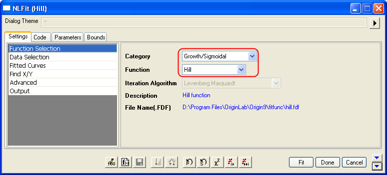
With the graph active, select the menu item Analysis: Fitting: Nonlinear Curve Fit to bring up the NLFit dialog. Select Hill function from Growth/Sigmoidal category on the Settings: Function Selection page.
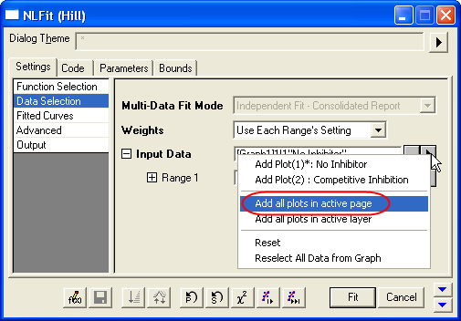
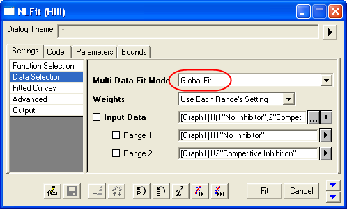
On the Settings: Data Selection page, click the triangular button next to the Input Data and choose Add all plots in active page to set the data range.
Select Global Fit from Multi-Data Fit Mode drop-down list on the Settings: Data Selection page.
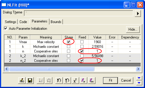
Switch to the Parameters tab, check the Share box on the Vmax row. These Share check boxes are only available when using Global Fit mode. Check the Fixed box for n and n_2, and make sure their values are 1.
Click the Fit button to generate the analysis reports. A table of fit parameters is pasted to the original graph (only the fit parameter values table is shown in the following figure.)

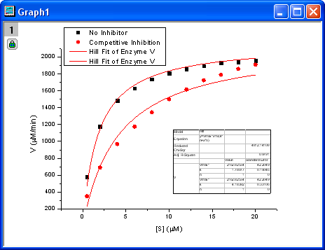
From the fit result, we can conclude that the maximum velocity is 2162.8 $\mu M/min$ . The value of $K_m$ for the no inhibitor model is 1.78 $\mu M$ . The value $K_m$ for the competitive inhibitor model is 4.18 $\mu M$ .

Fitting Lineweaver-Burk Plot

As we know, the model parameters can also be estimated by the Lineweaver–Burk or double-reciprocal plot. The Lineweaver–Burk plot takes the reciprocal of both sides of the M-M function and plots by 1/v vs. 1/[S]:

$\frac{1}{v}=\frac{1}{V_{max}}+\frac{K_m}{V_{max}[S]}$

This is actually a linear function:

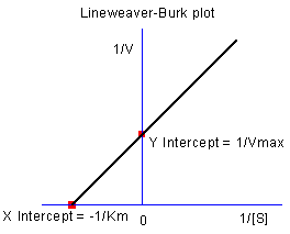
We will use the No Inhibitor data to illustrate how to calculate $K_m$ and $V_{max}$ by L-B plot.

Go back to the raw data worksheet and add two more columns by clicking the button. Right-click on column D and select Set As: X from the context fly-out menu to set it as an X column. Right-click on column D again and select Set Column Values to bring up the Set Values dialog. In the dialog edit box, enter: 1/Col(A) and set the Recalculate mode as None, since we don't need to auto update the reciprocal values in this example.
Similarly, set column E's values as 1/Col(B). Enter the long name for column D & E as $1/[S]$ & $1/V$ , respectively. And then we have:
Highlight columns D & E and click button to create a scatter plot.

From the above equation, we know there is a linear relationship between 1/v and 1/[S], so we can use the NLFit tool to fit a straight line on this plot. (You can also use the Fit Linear tool from Analysis: Fitting: Fit Linear)
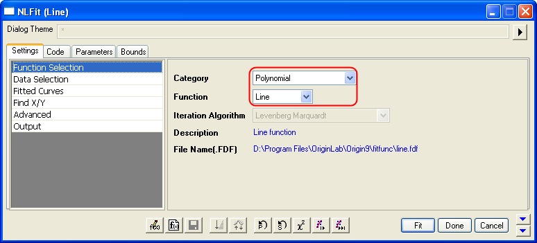
Bring up the NLFit dialog again, select Line function from Polynomial category, and then click the Fit button directly to generate results.

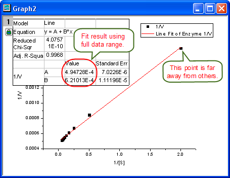
From the plot, one may doubt that this is the best fit curve since there is a point located far away. Actually, the right side of L-B plot is low substrate concentrations area, the measurement error may be large, so we'd better exclude these points during fitting.
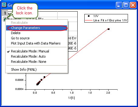
Click the lock icon on the graph upper-left corner, and select Change Parameters to bring back NLFit dialog.

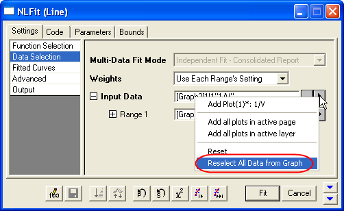
In Settings: Data Selection page, click the button on Input Data node, and then choose Reselect All Data from Graph from fly-out menu.

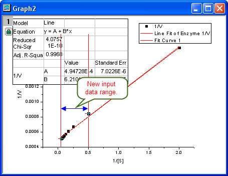
Then the NLFit dialog rolls up and your cursors become when you move to the graph page. Click and draw a rectangle to select data points you want to fit. The input range is labeled by vertical lines. You can also click-and-move these lines to change the input range.

Click the button on Select Data in Graph window to go back to NLFit dialog.
Click the Fit button on the NLFit dialog to recalculate the result. You can see from the graph that the report table was updated.
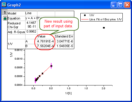
Since the intercept of the fitted curve is $1/V_{max}$ , it is equal to 4.76191E-4 in this example. To get the $V_{max}$ value, select Window: Command Window to open the command window, type
1/4.76191E-4 =

and press ENTER:

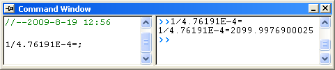Origin returns the value 2099, which is close to what we got above, 2160. (When fitting the hill function above, we shared $V_{max}$ when fitting two datasets. If you fit the No Inhibitor data only, this value will be closer.)