4.2.2.14 Fitting with Integral using LabTalk FunctionFitting-Integral-LabTalk
Summary
Since version Origin 8.6, Origin introduces a new LabTalk function, integral(), to do one-dimensional integration. This function returns the integral value of:
, dt")
And the interface of the integral() function is defined as below:
integral(integrandName, LowerLimit, UpperLimit [, arg1, arg2, ...])
Where integrandName here is the function name of the integrand:
\,")
In other word, the integral() function do the following things:
- Accept another function (the first argument) as the integrand.
- Perform integration on specified lower and upper limit and return the integral value.
- If need, pass the subsequent arguments (Arg1, Arg2, ...) into the integrand function.
Using this feature, we can define a fitting function with integral() function, and pass proper fitting parameters to the integrand, to do integration in curve fitting.
In this tutorial, we will modify the other tutorial, calling NAG functions to do integration during fitting, into LabTalk form, and show you how simple and straightforward to fit an integration function.
Minimum Origin Version Required: Origin 8.6
 | Beginning with Origin 2018b, you can define a an implicit function using integrals
|
What you will learn
This tutorial will show you how to:
- Create a fitting function using the Fitting Function Builder
- Create a fitting function with a Definite Integral using Labtalk function
- Set up the Initial Code for the fitting function
Example and Steps
The Fitting Model
The fitting model is described as below:
^2}{w^2}}, dt")
There are four parameters in the fitting function, and we need to pass three of them into the integrand, and use the independent variable as upper limit, to do integration. So you should define the integrand first, and then use the integral() function to perform integration inside your fitting function body.
Define the Function
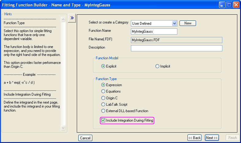
- Press F8 to open Fitting Function Builder dialog. Make sure choosing Create a New Function option, and click Next to navigate to the next page.
- In the Name and Type page, enter a function name, say MyIntegGauss. Leave the default function type as Expression, and then check the Include Integration During Fitting checkbox. This will lead you to a new page in the next step.
- In the Integrand page, you can define the expression of the integrand. Currently, Origin supports one-dimensional integral only, so the integrand should have ONE integration variable. In this example, the expression of the integrand is:
^2}{w^2}}")
The other variables, like xc, w, and A, are parameters of the integrand. To distinguish from fitting parameters, we named them Arguments here, and use the arguments name ixc, iw, and iA instead. Later, we can pass fitting parameters into these arguments. So, the integrand definition should looks like:
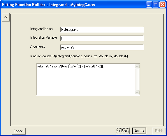
Note that this is a LabTalk function. To get the integration value, you must have a RETURN statement in the function body. And the integrand expression in this example should be:
return iA * exp(-2*(t-ixc)^2/iw^2) / (iw*sqrt(PI/2));
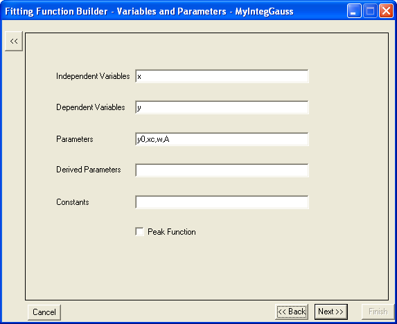
- When all set, click Next to go to the Variables and Parameters page to define the variables and parameters for the fitting function as below:
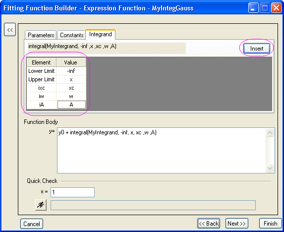
- The next Function page is where you define the fitting function body. Once you choose to include integration in your fitting function at the beginning of the fitting function builder wizard, there is an extra tab, Integrand, shown on this page. In this tab, you can map the fitting variables and parameters with elements of the integrand, including lower limit, upper limit, and integrand arguments. And in this example, we will map the variables as below:
| Integrand elements
|
Values pass into integrand
|
| Lower Limit
|
-inf
|
| Upper Limit
|
x
|
| ixc
|
xc
|
| iw
|
w
|
| iA
|
A
|
Once set up all the mappings as above table, click the Insert button, then well prepared integral() function is inserted into the Function Body box as:
integral(MyIntegrand, -inf ,x ,xc ,w ,A)
This expression means perform integration on the function, whose name is MyIntegrand, from negative infinite to x, and pass the three fitting parameters, xc, w, and A to the integrand.
By adding the constant parameter, y0, into the expression, the whole fitting function body should be:
y0 + integral(MyIntegrand, -inf, x, xc ,w ,A);
And the page may looks as below:
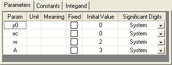
- Then active the Parameters tab, and give some proper initial values for each fitting parameters as:
Now, you can click Finish button to save this fitting function.
Fit the Curve
Copy and paste the following data into Origin worksheet:
| X
|
Y
|
| -1.69897
|
0.13136
|
| -1.22185
|
0.34384
|
| -0.92082
|
0.6554
|
| -0.82391
|
0.73699
|
| -0.69897
|
1.00157
|
| 0
|
1.70785
|
| 0.30103
|
2.31437
|
| 0.69897
|
2.77326
|
| 1
|
2.79321
|
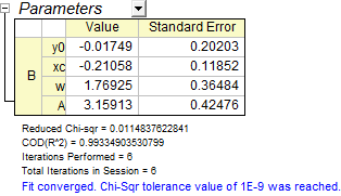
Highlight the Y column, and press Ctrl + Y to open the NLFit dialog. Select the function you just defined, and click Fit button to perform fitting. The fitting result should be the same like using NAG function directly:
|