4.2.2.28 Parameter Initialization for Rational FunctionsRationalFunc-InitialParameter
Summary
In this tutorial, we will show you how to calculate initial parameters for rational fitting functions using the multiple linear regression method, and perform a fit of the data using calculated initial parameters.
Minimum Origin Version Required: Origin 9.0 SR0
What you will learn
This tutorial will show you how to:
- Calculate initial parameters for rational fitting functions.
- Perform multiple linear regression using Origin C code.
Example and Steps
Algorithm
In this tutorial, we will use the following rational function as an example:

where x is the independent variable, y is the dependent variable, and a, b, c, d, e are fitting parameters.
Multiplying both sides by the denominator on the right side yields:

and the equation can be expressed as:

Substituting fitting data  \;\; i=1 \ldots N") into the equation gives: into the equation gives:

Hence estimating initial parameters for a rational polynomial fitting function becomes a multiple linear regression problem with linear coefficients a, b, c, d, e.

Origin provides a function ocmath_multiple_linear_regression in Origin C for multiple linear regression, which can be called in initialization code.
Import Data
- Open a new workbook.
- Copy data in Sample Data to the workbook.
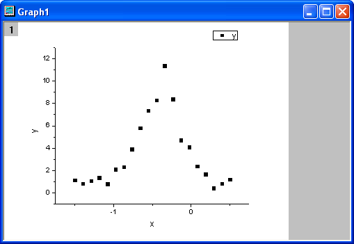
- Highlight column B, and select Plot: Symbol: Scatter from Origin menu. The graph should look like:
Define Fitting Function and Initialize Parameters
The fitting function can be defined using the Fitting Function Builder tool.
- Select Tools: Fitting Function Builder from Origin menu.
- In the Fitting Function Builder dialog's Goal page, click the Next button.
- In the Name and Type page, select User Defined from the Select or create a Category drop-down list, type rationalfunc in the Function Name field, and select Expression in the Function Type group. Click the Next button.
- In the Variables and Parameters page, type a, b, c, d, e in the Parameters field. Click the Next button.
- In the Expression Function page, type the following script in the Function Body box.
(a+b*x+c*x^2)/(1+d*x+e*x^2)
Click the Evaluate button, and it shows y=1 at x=1, hence this implies the expression is correct. Click the Next button.
- In the Parameter Initialization Code page, select Use Custom Code radio butto, click the Open Code Builder button
 to the right of the Initialization Code box, and initialize fitting parameters as follows, in terms of the algorithm. to the right of the Initialization Code box, and initialize fitting parameters as follows, in terms of the algorithm.
  UINT nOSizeN = x_data.GetSize(); //Number of points
  UINT nVSizeM = 5; //Number of parameters

  matrix mX(nOSizeN, 5);

  //Construct matrix for data points of independent variables
  vector vCa(nOSizeN), vCb, vCc, vCd, vCe;
  vCa = 1;
  mX.SetColumn( vCa, 0 );
  vCb = x_data;
  mX.SetColumn( vCb, 1 );
  vCc = x_data^2;
  mX.SetColumn( vCc, 2 );
  vCd = -x_data*y_data;
  mX.SetColumn( vCd, 3 );
  vCe = -x_data^2*y_data;
  mX.SetColumn( vCe, 4 );

  //Options for multiple linear regression
  LROptions stLROptions;
  stLROptions.UseReducedChiSq = 1;
  stLROptions.FixIntercept = 1; //Fix the intercept at 0.

  FitParameter stFitParameters[ 6 ]; // should be nVSizeM+1
  UINT nFitSize = nVSizeM + 1;

  int nRet = ocmath_multiple_linear_regression(mX, nOSizeN, nVSizeM, y_data,
    NULL, 0, &stLROptions, stFitParameters, nFitSize );

  if( nRet == STATS_NO_ERROR )
  {
    a = stFitParameters[1].Value;
    b = stFitParameters[2].Value;
    c = stFitParameters[3].Value;
    d = stFitParameters[4].Value;
    e = stFitParameters[5].Value;
  }
Click the Compile button to compile the code. And click the Return to Dialog button. Click Finish to close the Fitting Function Builder dialog.
Fit the Curve
- Select Analysis: Fitting: Nonlinear Curve Fit from Origin menu. In the NLFit dialog, select Settings: Function Selection, in the page select User Defined from the Category drop-down list and rationalfunc function from the Function drop-down list.
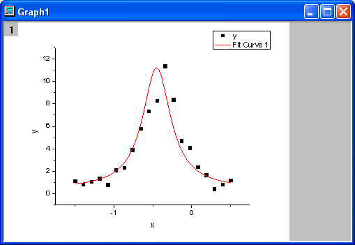
- Click the Parameters tab. Initial parameters calculated from initialization code are listed in the dialog, and the fitting function curve for initial parameters is shown as follows. It seems that initial parameters from initialization code are very good.
- Click the Fit button to fit the curve.
Fitting Results
The fitted curve should look like:
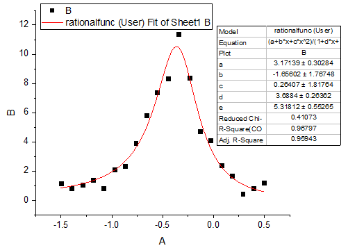
Fitted Parameters are shown as follows:
| Parameter
|
Value
|
Standard Error
|
| a
|
3.17139
|
0.30284
|
| b
|
-1.65602
|
1.76748
|
| c
|
0.26407
|
1.81764
|
| d
|
3.6884
|
0.26362
|
| e
|
5.31812
|
0.55265
|
Sample Data
| x
|
y
|
| -1.5
|
1.13173
|
| -1.39474
|
0.8262
|
| -1.28947
|
1.06999
|
| -1.18421
|
1.37155
|
| -1.07895
|
0.79569
|
| -0.97368
|
2.11346
|
| -0.86842
|
2.32006
|
| -0.76316
|
3.9205
|
| -0.65789
|
5.81904
|
| -0.55263
|
7.38037
|
| -0.44737
|
8.31272
|
| -0.34211
|
11.39718
|
| -0.23684
|
8.39808
|
| -0.13158
|
4.7305
|
| -0.02632
|
4.11105
|
| 0.07895
|
2.39105
|
| 0.18421
|
1.65394
|
| 0.28947
|
0.42953
|
| 0.39474
|
0.83337
|
| 0.5
|
1.18758
|
| Note: You can also use this method to initialize parameters for other rational polynomial fitting functions.
|
|