4.2.2.21 Fitting with Piecewise FunctionsFitting-Piecewise
Summary
We will show you how to define piecewise fitting function in this tutorial.
Minimum Origin Version Required: Origin 8.0 SR6
What you will learn
This tutorial will show you how to:
- Define piecewise (conditional) fitting functions.
Example and Steps
We can start this tutorial by importing the sample \Samples\Curve Fitting\Exponential Decay.dat data file. Highlight column D and plot a Scatter Graph. You can fit this curve using built-in functions under Growth/Sigmoidal category, however, in this tutorial, we will separate the curve into two parts by a piecewise function.
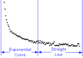
So the equation will be:

Define the Function
Press F9 to open the Fitting Function Organizer and define a function like:
| Function Name:
|
piecewise
|
| Function Type:
|
User-Defined
|
| Independent Variables:
|
x
|
| Dependent Variables:
|
y
|
| Parameter Names:
|
xc, a, b, t1
|
| Function Form:
|
Origin C
|
| Function:
|
|
Click the  button on the right of the Function edit box and define the fitting function in Code Builder using: button on the right of the Function edit box and define the fitting function in Code Builder using:
void _nlsfpiecewise(
// Fit Parameter(s):
double xc, double a, double b, double t1,
// Independent Variable(s):
double x,
// Dependent Variable(s):
double& y)
{
	// Beginning of editable part
	// Divide the curve by if condition.
	if(x<xc) {
		y = a+b*x+exp(-(x-xc)/t1);
	} else {
		y = a+b*x;
	}
	// End of editable part
}
Fit the Curve
Press Ctrl + Y to bring up NLFit dialog with the graph window active. Select the piecewise function we defined and initialize the parameter values:
Click Fit button to generate the results:
| xc:
|
0.24
|
| a:
|
36.76585
|
| b:
|
-24.62876
|
| t1:
|
0.04961
|
Note that this function is sensitive to xc and t1, different initial values could generate different results.
|