4.2.2.16 Fitting with SummationFitting-Summation
Summary
We have showed you how to perform fitting with an integral using the NAG Library, and now you'll learn how to do that without calling NAG functions. In this tutorial, we will show you how to do integration by the trapezoidal rule and include the summation procedure in the fitting function.
Minimum Origin Version Required: Origin 8.0 SR6
What you will learn
- How to include summation in your fitting function.
- Trapezoidal rule for integration.
Example and Steps
We will fit the same model as the integral fit using NAG:
^2}{w^2}}, dx")
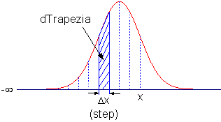
The difference is that we will perform the integration within the fitting function. Using the trapezoidal rule, we will first divide the curve into pieces and then approximate the integral area by multiple trapezoids. The precision of the result then depends on how many trapezoids will be used. Since this is a semi-infinite integration, we will set an increment (steps) and construct trapezoids from the upper integral limit, x, to the lower integral limit, negative infinity and then accumulate the area of these trapezoids. When the increment of the area is significantly small, we will stop the summation. Before doing the summation, you should guarantee that the function is CONVERGENT, or you should include a convergence check in your code.
Define the Function
Select Tools:Fitting Function Organizer or alternatively press the F9 key to open the Fitting Function Organizer and then define the function as follows:
| Function Name:
|
summation
|
| Function Type:
|
User-Defined
|
| Independent Variables:
|
x
|
| Dependent Variables:
|
y
|
| Parameter Names:
|
y0, A, xc, w
|
| Function Form:
|
Origin C
|
| Function:
|
|
Click the button (icon) beside the Function box to open Code Builder. Define, compile and save the fitting function as follows:
#pragma warning(error : 15618)
#include <origin.h>

// Subroutine for integrand
double f(double x, double A, double xc, double w)
{
	return A * exp(-2*(x-xc)*(x-xc)/w/w) / w / sqrt(PI/2);
}

//----------------------------------------------------------
//
void _nlsfsummation(
// Fit Parameter(s):
double y0, double A, double xc, double w,
// Independent Variable(s):
double x,
// Dependent Variable(s):
double& y)
{
	// Beginning of editable part
	// Set the tolerance for stop integration.
	double dPrecision = 1e-12;
	// Initialization
	double dIntegral = 0.0;
	double dTrapezia = 0.0;
	// Steps, or Precision.
	double dStep = 0.01;
	// Perform integrate by trapezoidal rule.
	// Note that you should guarantee that the function is CONVERGENT.
	do
	{
		// Trapezia area.
		dTrapezia = 0.5 * ( f(x, A, xc, w) + f((x-dStep), A, xc, w) ) * dStep;
		// Accumulate area.
		dIntegral += dTrapezia;
		x -= dStep;
	}while( (dTrapezia/dIntegral) > dPrecision );
	// Set y value.
	y = y0 + dIntegral;
	// End of editable part
}
Fit the Curve
We can use the same data to test the result.
- Import \Samples\Curve Fitting\Replicate Response Data.dat.
- Highlight the first column, right-click on it, and select Set Column Values from the context menu.
- Set
 = log(Col(A))") in the Set Column Values dialog. This will make a sigmoidal curve. in the Set Column Values dialog. This will make a sigmoidal curve.
- Highlight columns A and B and create a scatter plot.
- Then bring up the NLFit dialog by pressing Ctrl + Y. Select the fitting function we just defined and go to the Parameters tab, initialize all parameters to 1 and fit. You should see these results:
|
|
Value
|
Standard Error
|
| y0
|
-0.00806
|
0.18319
|
| A
|
3.16479
|
0.39624
|
| xc
|
-0.19393
|
0.10108
|
| w
|
1.7725
|
0.33878
|
|