4.2.2.20 Fit Function with Non-constant BackgroundFitting-with-Background
Summary
Many of the Origin built-in functions are defined as:

Where y0 can be treated as the "constant background". How about fitting a curve with a non-constant background? One option is to use the Peak Analyzer we provide. The Peak Analyzer includes multiple methods to subtract the baseline, including exponential or polynomial backgrounds. In this tutorial, we will show you how to fit such curves without using the Peak Analyzer.
Minimum Origin Version Required: Origin 8.0 SR6
What you will learn
Example and Steps
Prepare the Data
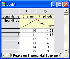
Let's start this tutorial by importing \Samples\Spectroscopy\Peaks on Exponential Baseline.dat. From the worksheet sparkline, we can see that there are two peaks in the curve. To simplify the problem, we will fit just one peak in this example.
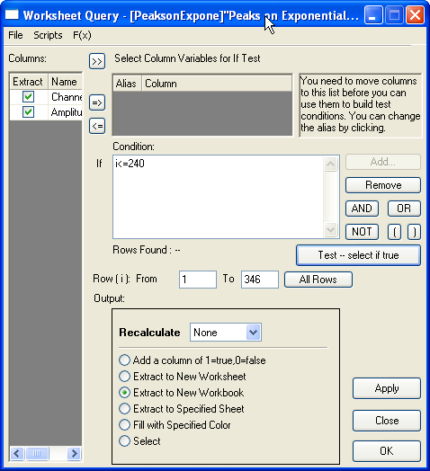
Now bring up the Worksheet Query dialog from Worksheet : Worksheet Query. And we will extract data from row 1 to row 240:
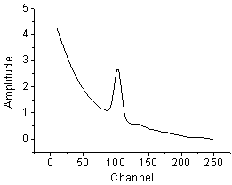
So the curve we will fit should look like this:
Define the Function
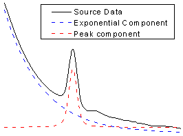
As illustrated below, we can consider the source curve is the combination of an exponential decay component (the background) with a Voigt peak:
So should we write down the whole equation to define the function? Like:
^2 + \left( \sqrt{4\ln{2}}\frac{x-x_c}{w_G}-t \right)^2}dt")
Well, this is a complicated equation and it includes infinite integration. Writing such an equation directly is painful. Now that we already have these two built-in functions:
ExpDec1:

Voigt:
^2 + \left( \sqrt{4\ln{2}}\frac{x-x_c}{w_G}-t \right)^2}dt")
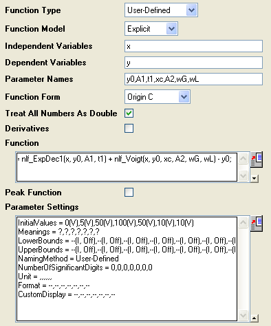
we can simply use the nlfxFuncName method to quote these two built-in functions and create a new one. Press F9 to open the Fitting Function Organizer and define a function as below:
| Function Name:
|
ExpVoigt
|
| Function Type:
|
User-Defined
|
| Independent Variables:
|
x
|
| Dependent Variables:
|
y
|
| Parameter Names:
|
y0, A1, t1, xc, A2, wG, wL
|
| Function Form:
|
Origin C
|
| Function:
|
y = nlf_ExpDec1(x, y0, A1, t1) + nlf_Voigt(x, y0, xc, A2, wG, wL) - y0;
|
Note:
Some of the built-in function names do not consistent with the actual DLL function name. Just like this Voigt function, it's defined in Voigt5.FDF, and if you open the FDF file by Notepad, you can see a line under [GENERAL INFORMATION] section says:
- Function Source=fgroup.Voigt5
The name after "fgroup" is the actual name we should put into nlf_FuncName.
Besides, for versions before Origin 8.1 SR2, the function body should use old nlfxFuncName notation and define as:
y = nlfxExpDec1(x, y0, A1, t1) + nlfxVoigt(x, y0, xc, A2, wG, wL) - y0;
x; xc; A1; t1; A2; wG; wL;
Listing the parameters at the end is done to avoid the "parameter not used inside the function body" error, although you already use these parameters. If not, you will not compile the function successfully.
|
Click the  button on the right of the Parameter Settings and enter these parameter initial values: button on the right of the Parameter Settings and enter these parameter initial values:
| y0:
|
0
|
| A1:
|
5
|
| t1:
|
50
|
| xc:
|
100
|
| A2:
|
50
|
| wG:
|
10
|
| wL:
|
10
|
So the final function definition part should look like:
Auto Parameter Initialization
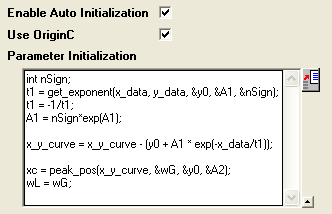
In the above section, we set fixed parameter initial values. If you know the possible fitted results, you can set the initial values in this way. But how about when the data is changed? Origin provides an Origin C interface to "guess" the initial values. To use the parameter initialization code, make sure to check the Enable Auto Initialization and Use OriginC checkboxes, and edit the code in Code Builder by clicking the icon.
(P.S: If you know the initial values very well, or you don't like coding, please skip this section.)
Now that the curve is composed by two components, we can guess the parameter values by separating these two parts, the initialization code includes:
- Use the get_exponent function to fit the curve and get the parameter values for exponential component.
- Remove the background -- exponential component -- from source data.
- Approaching the peak by Gaussian peak using peak_pos function and set the initial values for peak component
So, the initialization code in Code Builder should look like this:
void _nlsfParamExpVoigt(
// Fit Parameter(s):
double& y0, double& A1, double& t1, double& xc, double& A2, double& wG, double& wL,
// Independent Dataset(s):
vector& x_data,
// Dependent Dataset(s):
vector& y_data,
// Curve(s):
Curve x_y_curve,
// Auxilary error code:
int& nErr)
{
	// Beginning of editable part
	int nSign;
	// Evaluates the parameters' value, y0, ln(A) and R for y = y0+A*exp(R*x).
	t1 = get_exponent(x_data, y_data, &y0, &A1, &nSign);
	// Set the exponential component values for the fitting function.
	t1 = -1/t1;
	A1 = nSign*exp(A1);
	// Remove the exponential component from the curve;
	x_y_curve = x_y_curve - (y0 + A1 * exp(-x_data/t1));
	// Fit to get peak values.
	xc = peak_pos(x_y_curve, &wG, &y0, &A2);
	wL = wG;
	// End of editable part
}
| Note:
When you check the Enable Auto Initialization and enter the initialization code, this code will cover the initial values in Parameter Settings.
|
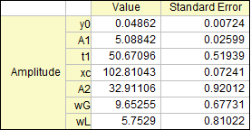
Fit the Curve
No matter what kind of parameter initialization method you used, highlight column B and press Ctrl + Y to bring up the NLFit dialog, select the ExpVoigt function and fit. The result should be:
|