4.2.2.26 Fitting with an Ordinary Differential EquationFitting-Ordinary-Differential-Equation
Summary
In this tutorial we will show you how to define an ordinary differential equation (ODE) in the Fitting function Builder dialog and perform a fit of the data using this fitting function.
Minimum Origin Version Required: Origin 9.1 SR0
What you will learn
This tutorial will show you how to:
- Define an ODE fitting function.
- Call NAG functions using Origin C code.
- Recalculate the ODE result only when parameters are updated.
- Interpolate on the ODE result.
Example and Steps
In this tutorial, we will use a first order ordinary differential equation as an example:
 
where a is a parameter in the ordinary differential equation and y0 is the initial value for the ODE. NAG functions d02pvc and d02pcc are called using the Runge–Kutta method to solve the ODE problem.
Import Data
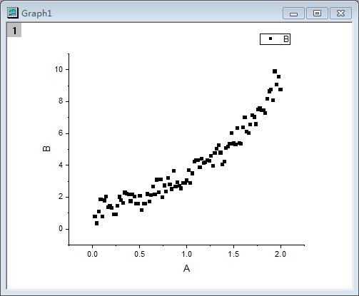
- Start with an empty workbook. Select Help: Open Folder: Sample Folder... to open the "Samples" folder. In this folder, open the Curve Fitting subfolder and find the file Exponential Growth.dat. Drag-and-drop this file into the empty worksheet to import it.
- Highlight B column, and select Plot: Symbol: Scatter from Origin menu. The graph should look like:
Define Fitting Function
The fitting function can be defined using the Fitting Function Builder tool.
- Select Tools: Fitting Function Builder from Origin menu.
- On the Fitting Function Builder dialog's Goal page, ensure the Create New Function radio button is selected. Click the Next button.
- On the Name and Type page, From the Select or create a Category drop-down list select User Defined. For Function Name type FitODE. In the Function Type section select the Origin C radio button. Click Next.
- On the Variables and Parameters page, in the Parameters field type a, y0. Click Next.
- On the Origin C Fitting Function page, click the
 button on the right of the Function Body edit box and define the function in Code Builder as follows.
Include header files for NAG and fitting: button on the right of the Function Body edit box and define the function in Code Builder as follows.
Include header files for NAG and fitting:
#include <oc_nag.h>
#include <ONLSF.H>
Define a static function to solve ODE by calling NAG functions. Call NAG function d02pvc to establish ODE model and d02pcc to solve the model:
struct user   // parameter in the ODE
{
	double a;
};

//Define the differentiate equation: y'=a*y
static void NAG_CALL f(double t, Integer neq, const double *y, double *yp, Nag_Comm *comm)
{
	neq; //Number of ordinary differential equations
	t; //Independent variable
	y; //Dependent variables
	yp; //First derivative

	struct user *sp = (struct user *)(comm->p);
	double a;
	a = sp->a;

	yp[0] = a*y[0];
}


//Use Runge-Kutta ODE23 to solve ODE
static bool nag_ode_fit( const double a, const double y0, const double tstart,
  const double tend, const int nout, vector &vP )
{
	//nout: Number of points to output
	if( nout < 2 )
		return false;

	vP.SetSize( nout );
	vP[0] = y0;

	int neq = 1; //Number of ordinary differential equations
	Nag_RK_method method;

	double hstart, tgot, tinc;

	double tol, twant;
	int i, j;

	vector thres(neq), ygot(neq), ymax(neq), ypgot(neq), ystart(neq);

	Nag_ErrorAssess errass;
	Nag_Comm comm;

	struct user s;
	s.a = a;
	comm.p = (Pointer)&s;
	ystart[0] = y0;
	for (i=0; i<neq; i++)
		thres[i] = 1.0e-8;
	errass = Nag_ErrorAssess_off;
	hstart = 0;
	method = Nag_RK_2_3;
	tinc = (tend-tstart)/(nout-1);
	tol = 1.0e-3;

	NagError nagErr1;
	//Setup ODE
	int iwsav[130];
	double* rwsav = (double*)malloc((350 + 32*neq)*sizeof(double));
	nag_ode_ivp_rkts_setup(neq, tstart, tend, ystart, tol, thres, method, errass, hstart, iwsav, rwsav, &nagErr1);

	if( nagErr1.code != NE_NOERROR )
	{
		free(rwsav);
		return false;
	}

	for (j=1; j<nout; j++)
	{
		twant = tstart + j*tinc;
		NagError nagErr2;
		//Solve ODE
		nag_ode_ivp_rkts_range(f, neq, twant, &tgot, ygot, ypgot, ymax, &comm, iwsav, rwsav, &nagErr2);

		if( nagErr2.code != NE_NOERROR )
		{
			free(rwsav);
			return false;
		}

		vP[j] = ygot[0];
	}

	free(rwsav);
	return true;
}
Define the fitting function body _nlsfFitODE:
NLFitContext *pCtxt = Project.GetNLFitContext();
if ( pCtxt )
{
  static vector vX, vY;
  static int nSize;

  BOOL bIsNewParamValues = pCtxt->IsNewParamValues();
  // If parameters were updated, we will recalculate the ODE result.
  if ( bIsNewParamValues )
  {
    //Initial and final values of the independent variable
    double tstart = 0.02, tend = 2, tinc;
    int nout = 100; //Number of points

    tinc = (tend-tstart)/(nout-1);
    vX.Data( tstart, tend, tinc );
    nSize = vX.GetSize();

    if( !nag_ode_fit( a, y0, tstart, tend, nout, vY) )
      return;
  }

  //Interpolate y from fitting data's x on the ODE result.
  ocmath_interpolate( &x, &y, 1, vX, vY, nSize );
}
Click the Compile button to compile the function body. To return, click Return to Dialog button. The Evaluate button on the dialog has a black figure of a running person. Clicking on it will show y=2.6627270424371. This implies that the function works. Click Next.
- In the Parameter Initialization Code page, select Use Custom Code radio button, and type the code in the Initialization Code box:
//Set the start y value in fitting data as the initial value of y0
y0 = y_data[0];
a = 1;
and click Finish.
| Note: In order to monitor the the fitted parameters, NLFitContext class was introduced in defining fitting function to achieve some key information within the fitter
|
Fit the Curve
- Highlight B column, then select Analysis: Fitting: Nonlinear Curve Fit from Origin menu. In the NLFit dialog, select Settings: Function Selection, in the page select User Defined from the Category drop-down list and FitODE function from the Function drop-down list.
- Select Parameters tab, and fix y0 as shown in the dialog.
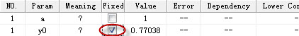
- Click Fit button to fit the curve.
Fitting Results
The fitted curve should resemble the following image:
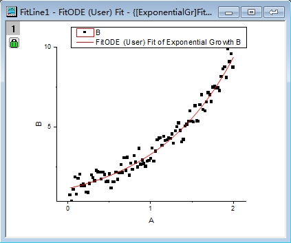
Fitted Parameters will be shown as in the following table:
| Parameter
|
Value
|
Standard Error
|
| a
|
1.30272
|
0.00858
|
| y0
|
0.77038
|
0
|
Note: Fitting with more complex ODE fitting functions can also be done in a similar way.
|