2.76 Generalized Linear Mixed Model(Pro)

GLMM

Summary

The Generalized Linear Mixed Model app is used to fit a generalized linear mixed model, which drops the normality and identity-link assumptions of Linear Mixed Effects Model and extend it to non-Gaussian and non-linear data.

Relative Topics: Linear Mixed Effects Model General Linear Model

Tutorial

Sample File

This tutorial uses the sample OPJU file shipped with the app. Right click the Generalized Linear Mixed Model app icon in the Apps Gallery (docked at the right side of Origin workspace), and choose Show Samples Folder from the context menu. In the folder that opens, drag-and-drop the project file Generalized Linear Mixed Model Sample.opju into Origin.

Note: If you want to save the OPJU after changing, it is recommended saving it to a different folder location (e.g. User Files Folder) or with a different name.

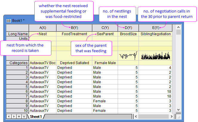
To study the begging behaviour of barn-owl nestlings, researchers collected negotiation calls during the 30s before a parent returned (column E in [Book1]Sheet1), and recorded the potential effecting factors including the nest locations (column A), food treatment - satiated or food-deprived (column B), sex of the feeding parent (column C), and brood size (column D). Generalized Linear Mixed Model is used to examine how these factors relate to the call rate.

Steps

1. Click the Generalized Linear Mixed Model app icon in the Apps Gallery to open the dialog.
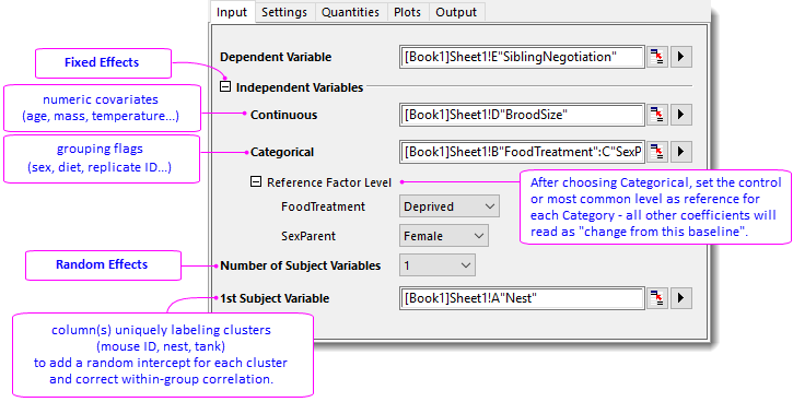
2. In the Input tab, set as follow:
   • Dependent Variable = Col(E)"SiblingNegotiation"
   • Continuous Variables = Col(D)"BroodSize"
   • Categorical Variables = Col(B)"FoodTreatment" and Col(C)"SexParent"
     • Specify Deprived and Female for Reference Factor Level of FoodTreatment and SexParenet, respectively.
   • 1st Subject Variable = Col(A)"Nest"

     

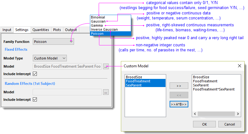
3. In the Settings tab, set as follow:
   • Family Function = Poisson
   • Under Fixed Effects group, choose Custom Model for Model Type, and then choose BroodSize, FoodTreatment, SexParent, FoodTreatment*SexParent in the popped-up dialog for Model.
   • Check Include Intercept checkbox for both Fixed and Random Effects.

   

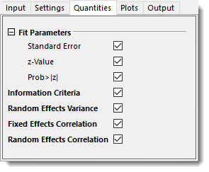
4. In the Quantities tab, check to output all the quantities.

   

5. In the Plots tab, check all plots.

   

6. Click OK.

Results and Explanations

• Fixed Effect Parameters Table

  

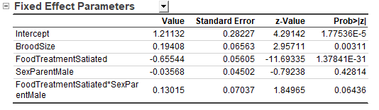
  • Intercept 1.21135 represents the predicted calls (in Log scale) which is used as a "reference" - supposing a brood of food-deprived nestlings fed by a female parent with brood size = 0 (a purely mathematical zero). That is, exp(1.21135) = 3.358 calls in 30s immediately before the adult arrives. This Intercept is considered the "baseline" and all the effects listed below (BroodSize, FoodTreament, SexParent) are calculated as deviations from it.
  • BroodSize: exp(0.19407) = 1.214 shows the call increment along with each additional nestling. That is, the call rate increases by 21.4% when every new nestling adds to the same nest, indicating intensified sibling negotiation as the brood size grows.
  • Similar, FoodTreatment = Satiated: exp(-0.65544) = 0.519. Satiated nestlings produce 48.1 % fewer calls than deprived ones, reflecting that hunger strongly amplifies begging.
  • SexParent = Male: exp(-0.03568) = 0.965 tells that calls are 3.5% lower when the father feeds. However, p = 0.42813 > 0.05 indicates no significant difference between male and female parents.
  • The last row is an interaction item, FoodTreatment*SexParent. p = 0.06437 > 0.05, therefore we drop the interaction term and keep the additive model only.
• Random Effect Summary
  • The Random Effect Parameter table quantifies how much call rates differ among nests after accounting for fixed effects.
  • The Random Effects Variance table calculates the variance of the nest-location intercept (Variance = 0.17188, SD = 0.41459). Using the latent-scale approximation for a Poisson-log, we roughly calculate ICC ≈ Variance / (Variance + 1) ≈ 0.172 / 1.172 ≈ 0.15, indicating that roughly 15 % of the residual variation is attributable to between-nest differences, while most variation rises within nest (the fixed effects).