2.75.2.1 Tutorial for Capability AnalysisTutorial-CA
Notes for Starting
- Download the sample project file from here and open it in Origin.
 | Topics for Further Reading:
|
Normal Capability Analysis
Background
A quality engineer wants to evaluate the pipe production process. He collected data for height (feet) of pipe at 150 samples.
He want to check whether the mean of the pipe height is 5 and the difference of their height can not vary more than 0.02 (4.98, 5.02)
Steps in Origin
- Open folder 1. Normal. Activate the workbook Height of Pipe.
- Highlight column A in worksheet. Click the Statistical Process Control icon
 in the Apps Gallery window. in the Apps Gallery window.
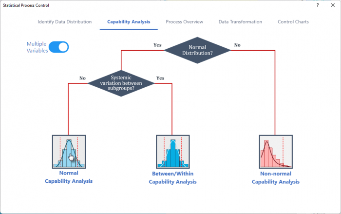
- Select the Capability Analysis tab, select Normal Capability Analysis
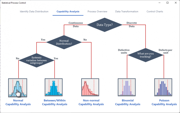
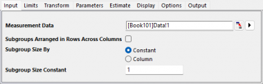
- In the Input tab of the opened dialog, column A is selected automatically as Measurement Data. Choose Subgroup Size By to be Constant and set the Subgroup Size Constant to be 1
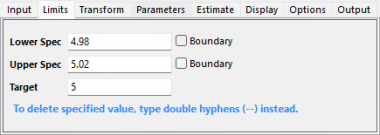
- In the Limits tab, set Lower Spec to be 4.98, Upper Spec to be 5.02 and Target to be 5
- Click OK button. A report sheet will be created
Interpreting the Results
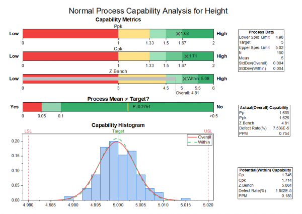
The process is approximately centered and all observed measurements are within the specification limits. The capability indices Cpk, Ppk, and Cpm are all greater than 1.33, which is a generally accepted minimum value for a capable process. Therefore, the width meets the production requirements
Between Within Capability Analysis
Background
A engineer wants to access the production process of the stainless steel sheet.
He collects 4 measurements of the thickness from 20 consecutive steel sheets. The thickness much be 3 ± 0.1 mm.
Steps in Origin
- Open folder 2. Between-Within, activate the workbook Steel Sheet
- Click the Statistical Process Control icon in the Apps Gallery window.
- Keep in the Capability Analysis tab, select Between/Within Capability Analysis
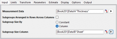
- In the Input tab of the opened dialog, select column A to be Measurement Data. Choose Subgroup Size By to be Column and set the Subgroup Size Column to be Column B
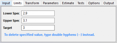
- In the Limits tab, set Lower Spec to be 2.9, Upper Spec to be 3.1 and Target to be 3
- Click OK button. A report sheet will be created
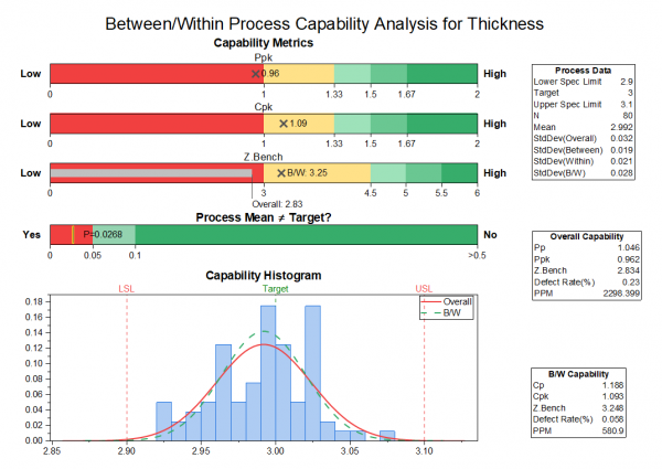
Interpreting the Results
Not all the measurements are within the specification limits. For between/within capability, Cp is 1.188, which indicates that the specification spread is 1.19 times greater than the 6-σ spread in the process. Cp and Cpk is a slightly different, indicating that the process is slightly off centered. For overall capability, Pp, Ppk, and Cpm are very close to each other, indicating that the process is centered and on target. However, Ppk is less than 1.33, which is a generally accepted minimum value for a capable process. We can conclude that the process is good but its capability still could be improved.
Non-normal Capability Analysis
Background
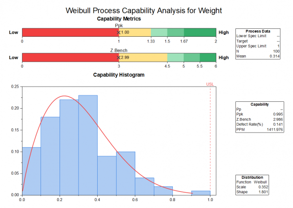
There is a dataset of weight values which follows the weibull distribution. We hope the data are not larger than 1.
Steps in Origin
- Opened folder 3. Nonnormal. Activate the workbook Weibull
- Click the Statistical Process Control icon in the Apps Gallery window.
- Keep in the Capability Analysis tab, select Non-normal Capability Analysis
- In the Input tab of the opened dialog, Measurement Data to be column A.
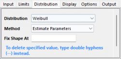
- In the Distribution' tab, set Distribution to be Weibull, set Method to be Estimate Parameters. Keep Fix Shape At box to be empty.
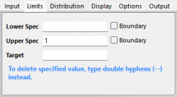
- In the Limits tab, set Upper Spec to be 1, keep all other text box to be empty.
- Click OK button. A report sheet will be created
Interpreting the Results
The dataset appear to follow the fitted curve of weibull distribution. All the measurements falls below the upper specification limits. We can say the process meets requirements
Binomial Capability Analysis
The binomial capability analysis is used to determine if the percentage of defective items in a process meets customer specifications. There are only two possible outcomes when you examine one item: it is either defective or not defective.
Background
The manager of a shop performs service satisfaction survey every day for 25 days and mark down the number of unsatisfied users.
He wants to know how well the service meets specifications.
Steps in Origin
- Opened folder 4. Binomial, activate the workbook Survey.
- Click the Statistical Process Control icon in the Apps Gallery window.
- Keep in the Capability Analysis tab, select Binnomial Capability Analysis
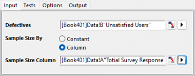
- In the Input tab of the opened dialog, set Defectives to be column B. Choose Sample Size By to be Column and set the Sample Size Column to be Column A
- Click OK button. A report sheet will be created
Interpreting the Results
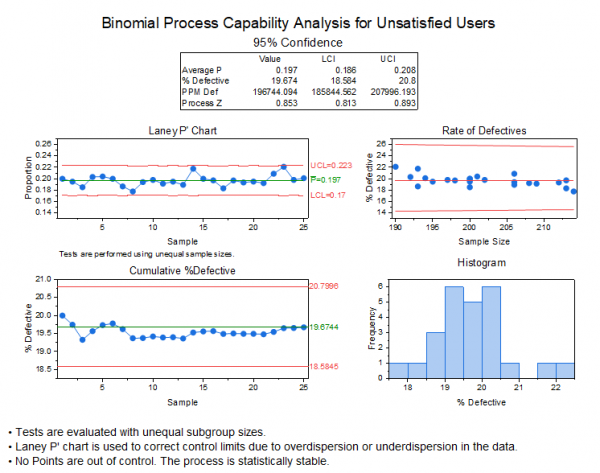
From the P chart we can see all samples fall within the control limit line, so overall it appears the process is in control. The Cumulative %Defactive Chart shows that, the estimated average percent of defects stabilizes at around 20%. In the Rate of Defectives plot, the points are randomly distributed around the average line.
In the Summary Stats table, the Process Z value is 0.853, it's much lower than 2. It indicates that the service does not meet the specifications. About 20% users are not satisfied with the service.
Poisson Capability Analysis
Background
We want to evaluate the plastic film production process. Data are collected once an hour on the plastic film. An area is cut out and the blemishes are counted. The area in
cm2 and the number of blemishes are recorded. We have recorded the data for the last 100 hours. We want to know whether the production meets requirements.
Steps in Origin
- Select the folder 5. Poisson in Project Explorer, activate the workbook Plastic Film
- Click the Statistical Process Control icon in the Apps Gallery window.
- Keep in the Capability Analysis tab, select Poisson Capability Analysis
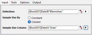
- In the Input tab of the opened dialog, set Defectives to be column B. Choose Sample Size By to be Column and set the Sample Size Column to be Column A
- Click OK button. A report sheet will be created
Interpreting the Results
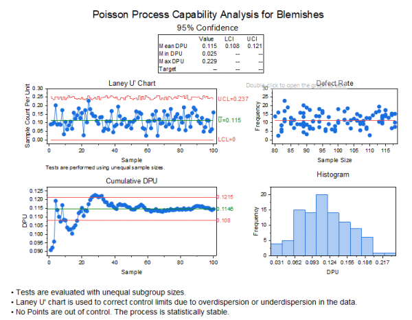
The U Chart assesses the state of statistical control of the results. There is one out-of-control point in the U Chart. Generally we can say the process is stable. The Cumulative DPU chart is used to determine if you have enough samples for a valid estimate of the average DPU. In the Cumulative DPU graph we can see data are flatten out along the average DPU line. That means we have enough samples to be sure that the estimated mean DPU is valid.
From the Summary Stats table, we can see the mean DPU (defects per unit) is 0.115. That is , there is 1 defect every 8.69 cm^2(1/0.115). The LCL and UCI are 0.108 and 0.121. That is, we are 95% confident that the mean DPU falls within the interval (0.108, 0.121).
Multiple Variables
Background
A manufacturer produces high-quality screw nuts that must equal 21 millimeters in diameter.
The quality control department drew 4 nuts from the finished products of two machines per day for 20 days, measured the diameters for each.
The analysis aims to: (1) test if the mean diameter equals 21 mm, (2) verify that Machine 1 outputs meet specifications (20.99–21.02 mm), (3) verify that Machine 2 outputs meet specifications (20.95–21.05 mm), and (4) monitor both machines' performance.
Steps in Origin
- Open folder 1. Normal. Activate the workbook Diameter.
- Highlight column B and C in worksheet. Click the Statistical Process Control icon in the Apps Gallery window.
- Select the Capability Analysis tab, select Multiple Variables check box and select Normal Capability Analysis
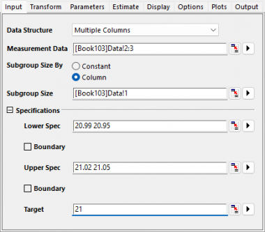
- In the Input tab of the opened dialog, column B and C is selected automatically as Measurement Data. Choose Subgroup Size By to be Column and set the Subgroup Size to be column A.
- Expand the Specifications branch, enter 20.99 20.95 in Lower Spec box, enter 21.02 21.05 in Upper Spec box. Enter 21 in the Target box
- Click OK button. A report sheet will be created
Interpreting the Results
The process is approximately centered and all observed measurements are within the specification limits. The capability indices Cpk, Ppk, and Cpm are all greater than 1.33, which is a generally accepted minimum value for a capable process. Therefore, the width meets the production requirements

|