2.2.5.1.1 Tutorial for ARIMA ToolTSA-ARIMA-Tutorial
Summary
In this sample, we will use ARIMA tool in Time Series Analysis app to fit monthly international airline passenger data with a specified model and forecast number of passenger in the next year.
Tutorial
This tutorial uses App’s built-in sample project. To open this sample OPJU file:
- Right click the Time Series Analysis App icon
 in the Apps Gallery and choose Show Samples Folder. in the Apps Gallery and choose Show Samples Folder.
- Drag-and-drop the project file TSA Sample.opju into Origin.
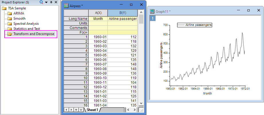
- Expand Project Explorer docked on the left. Select folder Transform and Decompose. The Sheet1 in Airpass Workbook represents monthly international airline passenger totals from 1960 to 1972. You can find this time series data with seasonality.
Pre-test
Before use ARIMA tool, we need to confirm parameters of the ARIMA model (p,d,q) (P,D,Q). Though the following test, you can get the parameters. For these tests, we have detail tutorial and you can click the link of them to know more detail. Here, we just show the brief steps.
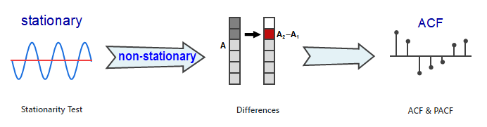
Stationary Test
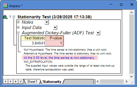
Before use ARIMA tool to analysis and forecast time series data, you need to do the Stationary Test to confirm the dataset is stationary. Usually, the dataset with trends or seasonality, that is a non-stationary time series.
In the result sheet, we can find the P-value>0.05, that means this time series data is non-stationary.
Difference
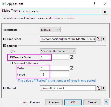
If the dataset is not stationary, you can use Differences tool to transform it to stationary. And the order of differencing is the Difference parameter for ARIMA model.
This data is non-stationary and seasonal dataset. Here, we set the Differences Order (d)=1,and Season Differences Order (D)=1, Period=12. Then you will get the stationary time series data in Column C.
Get the parameters
Using the stationary time series data in Column C, Autocorrelation and Partial Autocorrelation tool can help us to get the Autoregressive and Moving Average parameters.
Through the PACF result plot, we can get the non seasonal Moving Average (q) and Autoregressive (p). Also, through the ACF result plot, we can get the seasonal Moving Average (Q) and Autoregressive (P).
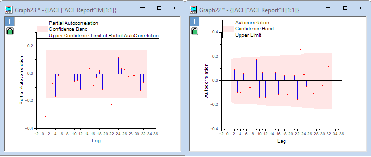
Finally, we confirm the ARIMA model (p,d,q) (P,D,Q) : (0,1,1) (2,1,0)
ARIMA
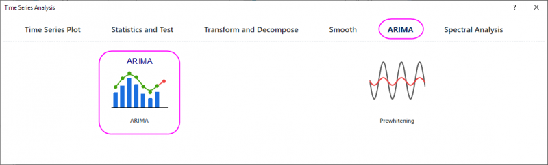
- Highlight the source data of Column B in the Worksheet. Click the Time Series Analysis App icon in the Apps Gallery.
- In the Time Series Analysis window, select ARIMA tab and then click ARIMA option to open the dialog.
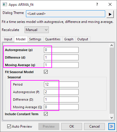
- Go to Model tab, check Fit Seasonal Model option. Then set the parameters:
- Autoregressive (p)=0
- Differences (d)=1
- Moving Average (q)=1
Seasonal:
- Period=12
- Autoregressive (P)=2
- Differences (D)=1
- Moving Average (Q)=0
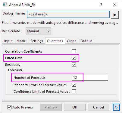
- Go to Quantities tab, select Fitted Data check-box and set the Number of Forecasts to 12.
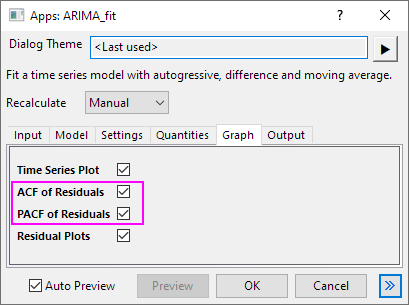
- Go to Graph tab, select ACF of Residuals and PACF of Residuals check-box. And click OK button to close the dialog.
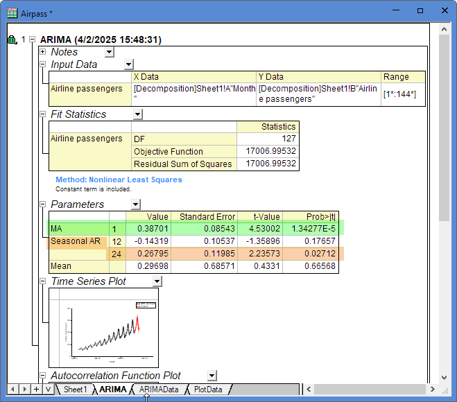
- In the result sheet, you can find the MA (Moving Average) term P-value<0.05, and Seasonal AR (Autoregressive) P-value<0.05. They are statistically significant.
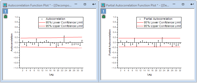
- Open the ACF and PACF Function Plots in the result sheet. You may see 1 or 2 significate correlations at higher order lags that are not seasonal lags. They are usually caused by random error. In this case, you can conclude that the residuals are independent.
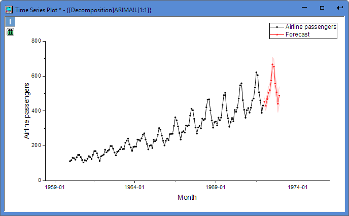
- We get the forecast result:
|