15.3.2.2 Settings Tab (Upper Panel)

See more related video:Selecting Data Range from Fitter

1 Function Selection
2 Data Selection
3 Fitted Curves
4 Find X/Y
5 Find Z
6 Advanced
7 Output

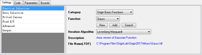
Function Selection

Select a fitting function using the drop-down lists.

Data Selection

Specify the input dataset and data modes.

Multi-Data Fit Mode
(only available with multiple range selections)

This control is available only when there is more than one input dataset.

Independent Fit - Consolidated Report
The input datasets are fitted separately. The reports are consolidated into one sheet. See Fitting Multiple Curves Independently for more information.
Independent Fit - Separate Report
The input datasets are fitted separately. The reports are output to different worksheets. See Fitting Multiple Curves Independently for more information.

Note: After you select an Independent Fit from the Multi-Data Fit Mode drop-down menu, the Independent Fit Drop-Down List list will appear in the row of buttons across the middle of the dialog. Select a dataset from this drop-down menu, and then click the 1 Iteration or Fit Until Converged button to the left of the menu.

Concatenate Fit
All input datasets are concatenated and fitted as one curve. Note that replicate data will not be combined before fitting but treated as individual data points. See Fitting with Replicate Data for more information.
Global Fit
All datasets are fitted globally. This mode should be used when you want to fit one model to multiple datasets with shared parameters. See: Global Fitting with Parameter Sharing.

Weights

Specify the weighting method. If Use Each Range's Setting is selected, the weighting method in the y sub-branch of each Input Data branch will be used when each range is fitted. Otherwise, the weighting method will be applied on all the input ranges.

Input Data

Specify the input dataset(s). Since Origin 2020b, if you started from a graph window, you can click the arrow button after this box to select Use X Scale Range to apply the X scale range on the source graph to the input range.

Range

The XY data range.

Worksheet

Specify the worksheet name of the dataset in a workbook.

X column of the curve.

Y column of the curve.

Weight

Weighting methods.

See: Fitting with Errors and Weighting

Rows

Specify a range of the X column to be fitted. When Rows is set to By Row or By X, you can use the From and To textboxes to specify the range to be fitted.

All

Specify all rows of the dataset to be fitted.

By Row

Specify the range of the X column by row index. Use To = 0 to specify "the last row" in the input data range.

By X

Specify the range of the X column by X value. The By X option supports use of a named range in place of actual X values. For more information, see this OriginLab blog post.

Fitted Curves

Show Preview on Source Graph

This control is available only when the input datasets are from a graph. When selected, fitted curves are previewed in the source graph.

Fitted Curves Plot

When selected, fitted curves will be output and other controls in this page will become available.

Plot in Report Table

When selected, fitted curves will be added to the Report Table.

Plot Type

This option is available only when the input datasets are from a graph and the Concatenate data mode is chosen. It can be used to control what is added to the source graph.

Raw Data
The combined input datasets are plotted.
Mean,SD
The mean values of the input datasets are plotted as scatter plot(s) with the standard deviations as error bars.
Mean,SE
The mean values of the input datasets are plotted as scatter plot (s) with the standard errors as error bars.

Note: When Mean, SD or Mean, SE is selected, a mean value that corresponds to an X value is calculated by averaging all the Y values from the input datasets, which correspond to the same X value. If there is only one Y value that corresponds to the X value, both SD and SE will be missing values.

Plot on Source Graph

This option is available only when the input datasets are from a graph. Use this to specify whether to add the fitted curve to the original graph.

None
The fitted curve is not added to the original graph.
Fitted Curve
The fitted curve is added to the original graph.
Fitted Curve+Plot Type
The fitted curve and the plot specified by the Plot Type drop-down list are added to the original graph. This option is available only when the input datasets are from a graph and the Concatenate Fit mode is chosen.

Stack with Residual vs.Indenpendents Plot

Stack the fitted curve with the Residual vs. Independents Plot.

Surface Plot Type

This option is available only when surface fit is used, and the fitted curve plot is enabled (in a report table, on a source graph, or both). It is used to specify the plot type for the fitted surface plot. Note that to add the plot for surface fitting results to a source graph, either OpenGL must be turned on, or the source graph must be created from XYZ worksheet data. See this table for details.

When OpenGL is turned on, the supported plot types are:

3D Surface
Contour

When OpenGL is turned off, the supported plot types are:

3D Colormap Surface
3D Color Fill Surface
3D Wire Frame
3D Wire Surface
Contour

Update Legend on Source Graph

This control is available only when the input datasets are from a graph. When selected, the legend of the input graph will be updated after the fitted curves are appended.

Multiple Plots Use Source Graph Color

This control is available only when the input datasets are from a graph and there is more than one input dataset. When selected, the color of the fitted curves is the same as the corresponding source plot.

X Data Type

Specify how to generate the X values of the fitted curve:

Same as Input Data
The X values of the fitted curve are the same as the input X values. It is the default option when Iteration Algorithm is set to Orthogonal Distance Regression.
Uniform Linear
The X values of the fitted curve are plotted on an equally-spaced linear scale.
Log
The X values of the fitted curve are plotted on a logarithmic scale.
Use Existing Dataset
Choose an existing dataset as the X values of the fitted curve. This option is not available for surface fit.
Follow Curve Shape
The X values of the fitted curve are smartly computed so that the fitted curve will follow the source curve shape. It is very useful when the shape of the source curve changes rapidly in some areas. It is the default option when Iteration Algorithm is set to Levenberg Marquardt.

Existing Dataset

This control is available only when X Data Type is Use Existing Dataset. It is used to select a dataset from the worksheet and use it as the X value of fitted curve. It must be a single data range (i.e. multiple range selections are not supported).

Points

This control is available only when X Data Type is either Uniform Linear or Log. It specifies the total number of data points in a fitted curve.

Range

This control is available only when X Data Type is either Uniform Linear or Log. It specifies the range of the X values of the fitted curve. Select one of the following options:

Use Input Data Range + Range Margin
Span to Full Axis Range
Custom

Range Margin

This control is available only when X Data Type is either Uniform Linear or Log, and Use Input Data Range + Range Margin is selected for Range. It specifies the range margin into which the fitted curves extend.

Min/Max

This control is available only when X Data Type is either Uniform Linear or Log, and Custom is selected for Range. These two text boxes specify the minimum and maximum X values for fitted curves.

Confidence Bands

Add confidence bands to the fitted curve plot as two lines with filled area in between. You can turn the area fill off or customize the fill pattern on the Line tab of Plot Details dialog.

Prediction Bands

Add prediction bands to the fitted curve plot as two lines with filled area in between. You can turn the area fill off or customize the fill pattern on the Line tab of Plot Details dialog.

Confidence Level for Curves (%)

Enter a confidence level for confidence bands and prediction bands.

Residual Plots

Use the controls in this branch to customize the residual plots.

When fitting with the Levenberg Marquardt algorithm:

Residual Type

Specify the residual type from the drop-down list:

Regular
Standardized
Studentized
Studentized Deleted

For the selected residual type, you can opt to output up to six residual plots:

Residual vs. Independents Plot

Histogram of the Residual Plot

Residual vs. Predicted Values Plot

Residual vs. the Order of the Data Plot

Residual Lag Plot

Normal Probability Plot of Residuals

For more details please see: Graphic Residual Analysis.

When fitting with the Orthogonal Distance Regression algorithm, there is only one option:

Residual Scatter Plot

Find X/Y

Control output of Find Specific X/Y tables. A Find Y from X table is used to obtain a dependent variable value that corresponds to a given independent variable value. Use a Find X from Y table to obtain an independent variable value for a given dependent variable value.

See: Finding Y/X from X/Y Standard Curves.

Find X from Y	Generate a Find X From Y table. Number of X Columns Specify the number of X columns.
Find Y from X	Generate a Find Y From X table. Number of Y Columns Specify the number of Y columns.

Note: This branch is disabled for nonlinear implicit curve fitting.

Find Z

This option is only available for surface fitting. Controls output of the Find Z from XY table. A Find Z from XY table is used to obtain a dependent variable value Z that corresponds to a set of given independent variable values X and Y.

Find Z from XY	Use the checkbox to specify whether to generate a Find Z from XY table. Number of Z Columns Specify the number of Z columns.

Advanced

Replica

Use these controls to fit your data to a built-in peak function by replicating the function for each peak, each of which may have different parameters. Your data should display multiple peaks of the same general form (e.g. Lorentzian or Gaussian) but with different centers or widths. If the function you have selected does not support replicas, this branch is disabled.

Number of Replicas

Specify the number of replicas. You must set the number to n-1, where n is the number of peaks you believe to be present in your data.

Peak Finding Settings

Settings related to peak finding.

Peak Finding Method for Nonlinear Curve Fit

Specifies the method to search peaks. Please see the Find Peaks page in the Peak Analyzer chapter for more details.

Local Maximum
Window Search
1st Derivative
2nd Derivative (search Hidden peaks)
Residual after 1st Derivative (search Hidden peaks)

Local Points(%)

Only available when Local Maximum is selected in the Method drop-down list. Controls the number of points (local area) used for finding the peaks with the Local Maximum method.

Window Height(%)

Only available when Window Search is selected in the Method drop-down list. Controls the height of the rectangle used to find peaks. Edit the Height value in the text box.

Window Width(%)

Only available when Window Search is selected in the Method drop-down list. Controls the width of the rectangle used to find the peaks. Edit the Width value in the text box.

Peak Finding Method for Nonlinear Surface Fit

Specifies the method to search peaks.

Local Maximum
1st Partial Derivative
Contour Consolidation

Local Points

Controls the number of points in the X and Y directions (local area), used for finding peaks.

Peak Direction

Narrow the search for positive and/or negative peaks.

Positive
Find positive peaks only.
Negative
Find negative peaks only.
Both
Find both positive and negative peaks.

Peak Min Height(%Y Scale)

Control the minimum height of the found peaks. For Nonlinear Surface Fit, the label will read Peak Min Height(%Z Scale).

Replicate From nth Parameter

Specify which parameters to use for fitting multiple peaks. For example, in a Gaussian function, the parameters are ordered y0, xc, w, and A. If set to 2, Origin will start with the second parameter when replicating. The first parameter will have only one value, so y0 will remain common for all replicas. Similarly, z0 would be common for surface peak replicas.

Number of Parameters Used in Replicas

The number of parameters used in replicas.

Plot Individual Peak Curve

Available for Nonlinear Curve Fit. Specify whether or not to plot the fitted curve for each individual peak.

Plot Cumulative Fitted Curve

Plot the cumulative fitted curve. Becomes available when Plot Individual Peak Curve is checked for Nonlinear Curve Fit. It will be checked (and non-editable) for Nonlinear Surface Fit.

See: Fitting Multiple Peaks with Replicas

Fit Control

Use this tree to control the fitting process.

Iterations

Control of iteration properties during fitting.

Max Number of Iterations

Specify the max number of iterations performed when the Fit button is clicked. If the Tolerance condition cannot be satisfied after the given maximum number of iterations are performed, user may press Fit again. The same number of iterations will be performed. This option prevents the fitting operation from running too long if each iteration is very slow (when data is large or when there are many parameters).

Tolerance

Specify the tolerance in this box. Fitting will be viewed as complete if the reduced chi-square between two successive iterations is less than the tolerance value. The tolerance is calculated by:
$Tolerance = \left | \frac{{\chi^2}'-\chi^2}{{\chi^2}'+\chi^2} \right |$
Where $\chi^2$ is the chi-square value of current iteration, and ${\chi^2}'$ is the chi-square of the last iteration. Note that a small chi-square tolerance does not necessarily mean that the fit is good. If the parameter space is “flat” (a particular combination of large variation of parameters could cause only a change of the chi-square value. This is similar to over-parameterization), then one cannot say that the fit is good even if the chi-square tolerance is satisfied.

Derivative Delta

This branch determines how the fitter computes the partial derivatives with respect to parameters for user-defined functions during the iterative procedure. This option is unavailable for built-in functions.

Note: You can define a user-defined function with partial derivatives.

For the user-defined functions, the derivative with respect to the parameter, p1, is computed as follows:

$derivative=[f(x,p_1+Delta,p_2,...)-f(x,p_1,p_2,...)]/Delta$ where $Delta$ is the increment.

Note: for simplicity, we suppose that the function has only one independent variable here.

Delta

The increment.

Minimum

Min value of the actual Delta. This text box is disabled when the Fixed check box is selected.

Maximum

Max value of the actual Delta. This text box is disabled when the Fixed check box is selected.

Fixed

Use fixed Delta value.

If the Fixed check box is selected, the value entered in the Delta text box will be used as the delta values for all the parameters.

If the Fixed check box is cleared, the actual value of Delta for a particular parameter will be equal to the product of the current value of the parameter and the value specified in the Delta text box. In this case, you can use the Maximum and Minimum text boxes to limit the actual Delta values in case a parameter value becomes too large or too small.

Note: It is not recommended that you select the Fixed check box when you start fitting your new function.

Parameters CI Computation Method

Use this list to select the method to compute the parameters confidence intervals:

Asymptotic-Symmetry based
With the Asymptotic-Symmetry method, you will get asymptotic, symmetrical confidence intervals as calculated by a related equation.
Model-Comparison based
If the Model-Comparison method is used, the upper and lower confidence limits will be calculated by comparing the residual sum of squares.

See: Theory of Nonlinear Curve Fitting.

Scale Error with sqrt(Reduced Chi-Sqr)

Available when fitting with weight. This check box only affects the error on the parameters reported from the fitting process, and does not affect the fitting process or the data in any way. It is enabled by default and the covariance matrix is calculated as: $\sigma^2(F'F)^{-1}$ , otherwise, $(F'F)^{-1}$ .

When it is checked, it Scale Error with sqrt reduced Chi-Sqr to estimate error variance, and parameter's standard error is scaled by it, otherwise error variance is specified with 1, and parameter's standard error is not scaled.

This option is checked by default to keep parameter's standard error and related results compatible with other software. It is recommended to uncheck this option when fitting data with instrumental weight, so that parameter's standard error can reflect the magnitude of weight.

Invalid Weight Data Treatment

Treat as Invalid

If there is invalid value in weight data, Origin will throw an error.

Replace with Custom Value

Replace the Invalid Weight data with Custom Value

Custom Weight

Set the value of Custom Weight. This option is available when Replace with Custom Value is selected.

Quantities

Control the quantities to be computed and displayed.

See: Theory of Nonlinear Curve Fitting

Fit Parameters

Use this branch to specify what is output to the Fit Parameters table of the report sheet.

Meaning

When this box is checked, a Meaning column is added to Parameters table in the result sheet (note that these will will be the same as those used in the Parameters table of the NLFit dialog). This box is unchecked by default.

Unit

The unit for parameters. If you checked this check box, a column "Unit" will be added into the Parameters table of the result sheet. The units defined in the Derived Parameter Settings box of the Fitting Function Organizer dialog will be shown in this column.

Value

The parameter values.

Fixed

Fix a parameter value.

Standard Error

The standard error of each parameter.

LCL

The lower confidence limit. The LCL results will be calculated for both parameters and derived parameters if there is any.

UCL

The upper confidence limit. The UCL results will be calculated for both parameters and derived parameters if there is any.

Confidence level for Parameters (%)

The confidence level for regression. This control is available only when either LCL or UCL is checked.

t-Value

The t-test value of parameters.

Prob > |t|

The p-value of parameters.

Dependency

The dependency values for parameters.

Cl Half-Width

The half-widths of the confidence intervals.

Lower Bound

Minimum parameter value.

Upper Bound

Maximum parameter value.

Fit Statistics

Control output to the Fit Statistics table of the report sheet.

Number of Points

The total number of input data points.

Degrees of Freedom

Model degrees of freedom.

Reduced chi-Sqr

The reduced chi square value.

R Value

The R value, equal to the square root of $R^2$ .

Residual Sum of Squares

The residual sum of squares (RSS), or the sum of square error.

R-Square (COD)

The coefficient of determination.

Adj. R-Square

The adjusted coefficient of determination.

Root MSE(SD)

The residual standard deviation, or square root of mean square error.

Number of Iterations

The number of iterations required for the fit to run to completion.

Fit Status

Any fit status error code that is generated. You can see this Quick Help topic for details.

Number of Replicas

The number of replicas.

Replicas From nth Parameter

The index number of the starting parameter used to generate replicas.

Number of Parameters Used in Replicas

The number of parameters used to generate replicas.

Fit Summary

Control output of the fit summary table. When selected, options include Value, Standard Error, LCL, UCL, Adj.R-Square, R-Square(COD),Reduced Chi-Sqr.

ANOVA

Output the analysis of variance table.

Covariance Matrix

Output the covariance matrix.

Correlation Matrix

Output the correlation matrix.

Residue Analysis

Options for output of residuals. See: Graphic Residual Analysis

Output

Use the Output Results To branch to control results output.

Graph	Specify the arrangement of graph. Results Table Specify whether to show the fitting results to the source/report graph. None No not add fitting result table to the graph. Source Graph Add fitting result table to the source graph. Make sense only when the input data is from graph. Report Graph Add fitting result table to the embedded graphs in the report sheet. When there are more than one graphs in the report sheet, the table will be added to the first one. Source and Report Graphs Add fitting result table to both the source graph and report sheet graph. Table Style Template Specify the Table Style Template used in the results graph. Quantities in Table Specify the quantities to display in table Custom Display for Error Value Table Specify the decimal digits for Error value in the result table on the graph Arrange Graphs into Columns Specify a number l. In any result sheet table, graphs will be arranged in rows of l graphs. Arrange Plots of same Type in One Graph If this check box is selected, plots of same type will be arranged in one graph. Arrange Residual Plots in One Graph If this check box is selected, residual plots will be arranged in one graph.
Dataset Identifier	Specify how to label the source data in your output. Specify the identifier for the source datasets. Identifier Select a type to specify the source datasets information. The Identifier can be Range, Book Name, Sheet Name, Name (Use the long name of the corresponding column if there is a long name, otherwise use the short name of column.), Short Name, Long Name, Units, Comments, <Custom> (For its usage, please refer to Advanced legend text customizations). Designation Specify using the X dataset, Y dataset etc. to provide the Identifier. Choosing <auto> uses the dependent variable (typically, the Y column). This control is not available for all identifiers. Show Identifier in Flat Sheet Many Origin analysis operations output data to a "flat" sheet in addition to the collapsible analysis report sheets. Use the Identifier in the flat sheet.
Fitted Results Sheet Arrangement	Control arrangement of fitted result worksheets. List is only available when the multiple datasets are inputted and the Multi-Data Fit Mode is Independent Consolidated Report. Combined All results are combined in the worksheet. Separate The results are output to separate worksheets.
NLFit Tables	Control output of worksheet report tables. See: Output Results
Fitted Curves	Specify the destination workbooks and worksheet for the fitted value. See: Output Results
Fit Residuals	Workbook and worksheet to contain residual values. See: Output Results
Find Specific X/Y Tables	Determine where to output Find Specific X/Y tables. Available when either Find X from Y or Find Y from X is selected. in the Find Specific X/Y section below See: Output Results
Optional Report Tables	Specifies what is output to report worksheet optionally. Equation in Notes Specify the format of the equation on the report table. Equation with Names Output the equation with parameter names. Equation with Values Output the equation with the fitted values of parameter. Notes Notes table. Input Data Table for input data. Masked Data Table for masked data. Missing Data Table for missing data.