15.3.1 Quick StartNLFit-QuickStart
The nonlinear curve fitting (NLFit) tool includes more than 200 built-in fitting functions, selected from a wide range of categories and disciplines. If the function you are seeking for is not included, you can always define your own function using Origin's flexible Fitting Function Builder.
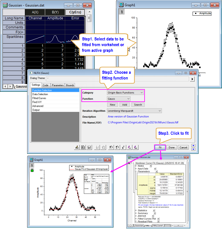
Specify Your Input Data
Origin permits you to pre-select input data from a worksheet or directly from a graph before opening NLFit dialog. Once you opened the NLFit dialog, you can also change, add, remove or reset the data from the Input Data Branch in Data Selection page under Settings tab.
Select Data from Worksheet
You can select data from one or more worksheet columns, parts of worksheet columns or even non-contiguous portions of worksheet columns. Hold Ctrl key when you want to make non-contiguous selection.
Select Data from Graph
When a graph window is active, the active curve in the active layer will be pre-selected as input for fitting.
Following options are available for other data pre-selection cases:
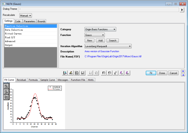
Fit with Built-in Functions
Origin built-in fitting functions includes automatic parameter initialization code that adjusts initial parameter values to your dataset(s), prior to fitting.
With just a few clicks, you can perform curve fitting and obtain "best-fit" parameter values. You can opt to have the best fit curve pasted to your original data plot:
- Highlight the data in worksheet or activate the graph window you want to fit, and choose Analysis: Fitting: Nonlinear Curve Fit menu to open NLFit dialog.
- Navigate in Category and Function drop-down lists to select a built-in fitting function.
- If a built-in function is not found, click Search to open Search Fitting Functions where you can search by keyword and load functions (see the tip below).
- Click Fit button to perform the fit and get result worksheets.
 |  When clicking on the Search button, you will notice an icon for the Fitting Function Library App in the upper-right corner of the Search dialog . Click on the icon to browse a list of downloadable functions. Alternately, if you search functions by keyword and no function is found, you will again have the chance to open the Library App and browse for an add-on function. Note that this App is preinstalled in the latest versions of Origin. When clicking on the Search button, you will notice an icon for the Fitting Function Library App in the upper-right corner of the Search dialog . Click on the icon to browse a list of downloadable functions. Alternately, if you search functions by keyword and no function is found, you will again have the chance to open the Library App and browse for an add-on function. Note that this App is preinstalled in the latest versions of Origin.
|
Common Nonlinear Fits with Built-in Functions
In order to facilitate users to do some typical nonlinear fitting tasks with NLFit tool, Origin provides many quick menu entrances under the main menu Analysis: Fitting:
Implicit Curve Fit
Select Analysis: Fitting: Nonlinear Implicit Curve Fit menu to open the NLFit tool with the function category Implicit selected. You can check this example to see how to do a quick implicit fit.
Surface Fit
Select Analysis: Fitting: Nonlinear Surface Fit menu to open the NLFit tool with the function category Surface selected. You cam check this tutorial to learn how to do a surface fit quickly.
Exponential Fit
Select Analysis: Fitting: Exponential Fit menu to open the NLFit tool with the function category Exponential selected. You can check this example to see how to do a quick exponential fit.
Single Peak Fit
Select Analysis: Fitting: Single Peak Fit menu to open the NLFit tool with the function category Peak Functions selected. You can check this example to see how to do a quick peak fit with one peak function.
Sigmoidal Fit
Select Analysis: Fitting: Sigmoidal Fit menu to open the NLFit tool with the function category selected. You can check this example to see how to do a quick sigmoidal fit.
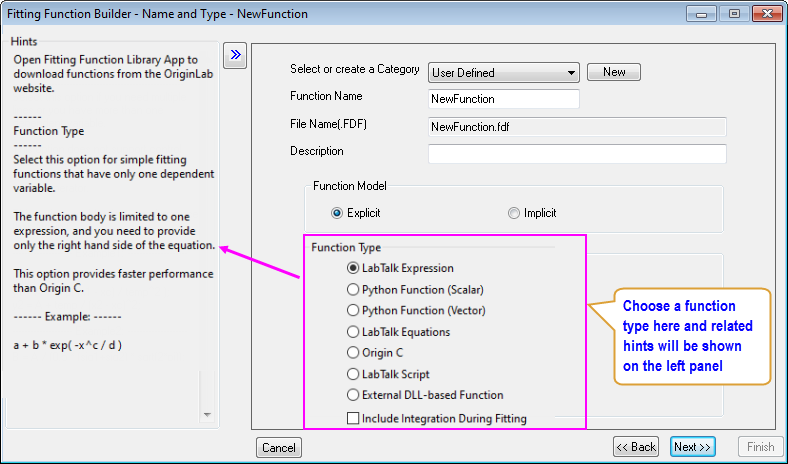
Fit with User-defined Functions
Can't find a suitable fitting function in our built-in function library? No problem. Our Tools: Fitting Function Builder can guide you step-by-step to define custom fitting functions easily.
Fit with Multiple Datasets
Do you have multiple datasets that you would like to fit simultaneously? With Origin, you can fit each dataset separately and output results in separate reports or in a consolidated report. Alternately, you can perform global fitting with shared parameters; or perform a concatenated fit which combines replicate data into a single dataset prior to fitting.
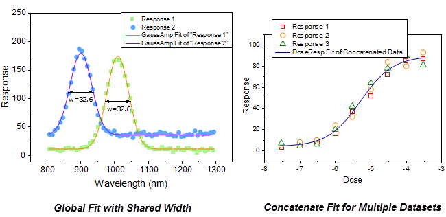
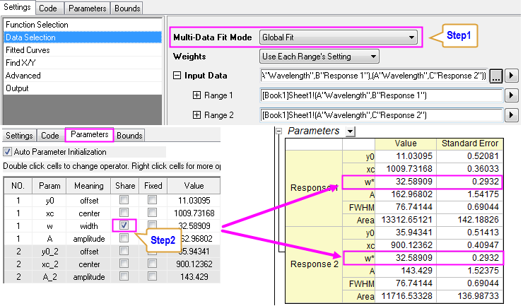
Global Fit with Shared Parameter
Parameters in the fitting function can optionally be shared amongst all datasets.
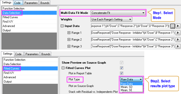
Concatenate Fit for Replicate Data
For replicate data, you can choose to concatenate all data points into one curve and fit them as a whole dataset.
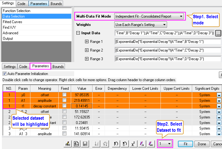
Independent Fit for Multiple Curves
You can choose to fit multiple curves independently. The independent fitting of multiple curves can be performed one by one to create Separate Report for each curve or simultaneously to generate a Consolidated Report.
Fitting Controls
Need to fine-tune your curve-fitting analysis? With Origin, you have full control over the curve-fitting process.
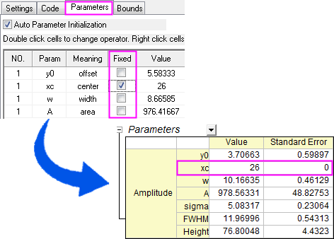
Fix Parameters
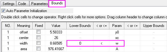
Set Upper and Lower Bounds
Set Linear Constraints
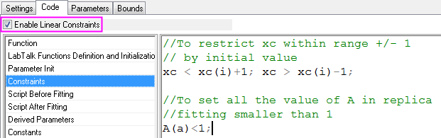
| Go to this table to learn how to write linear constraints.
|
Advanced Fitting Options
In addition to the basic fitting options, you also have access to extended options for more advanced fitting.
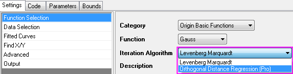
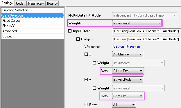
Fitting with X and Y Errors
Step 1. Choose Orthogonal Distance Regression iteration algorithm.
Step 2. Choose appropriate weighting methods.
Fit with Replicas
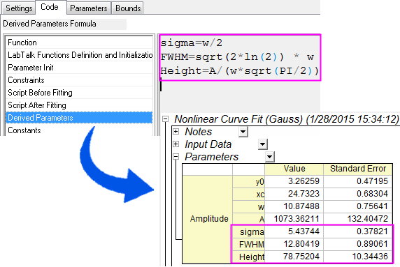
Obtain Derived Parameters
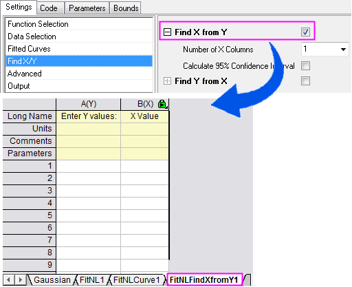
Find Y from X
Examples
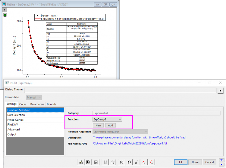
Fit Exponential Fucntions
- Highlight data and go to menu Analysis: Fitting: Exponential Fit.
- Select the fitting function ExpDecay3 from Function drop-down list.
- Click Fit button.
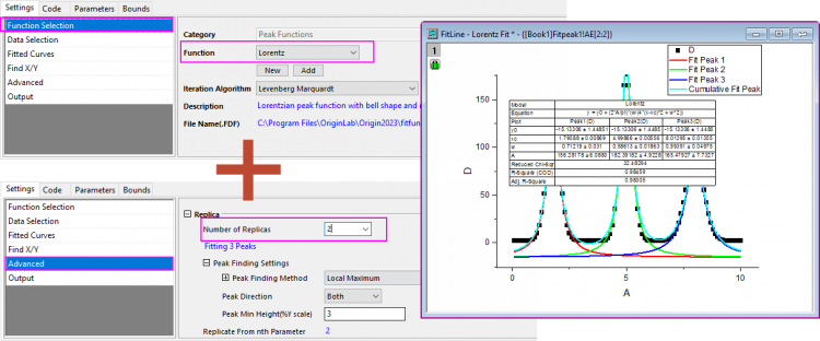
Fit Single Peak
- Highlight data and go to menu Analysis: Fitting: Fit Single Fit.
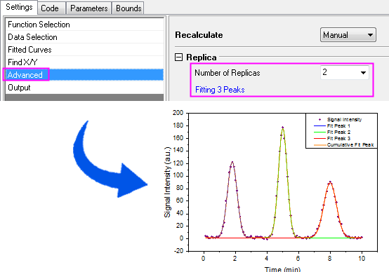
- Select the fitting function Lorentz from Function drop-down list in the Function Selection sub-tab. And go to the Advanced sub-tab, set Number of Replicas to 2 as there are three peaks in the curve, we can fit them with Replicas.
- Click Fit button.
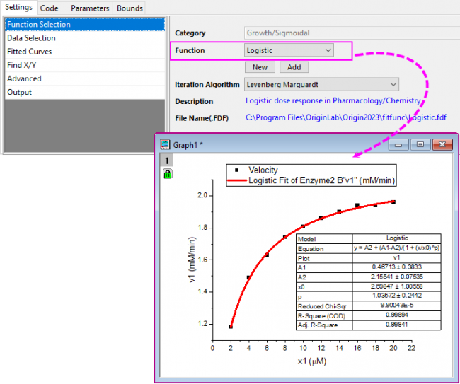
Fit Sigmoidal Functions
- Highlight data and go to menu Analysis: Fitting: Sigmoidal Fit.
- Select the fitting function Logistic from Function drop-down list.
- Click Fit button.
Fit Implicit Functions
- Highlight data and go to menu Analysis: Fitting: Nonlinear Implicit Curve Fit....
- Select fitting function from Function drop-down list.
- Click Fit button.
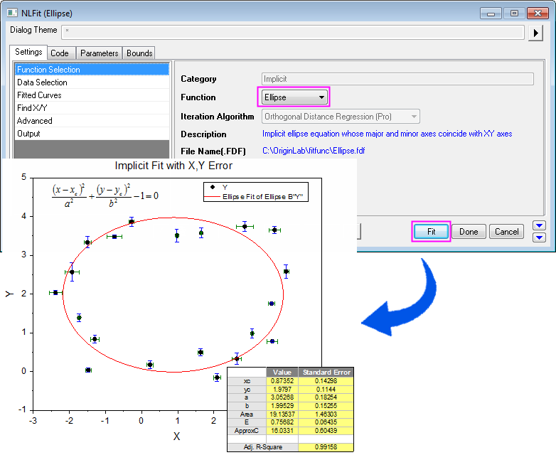
Read this tutorial to know how to define an implicit fitting function.
Fit with Integrals
Want to know what kind of integration function can be fitted and how to define your own fitting function?
Case 1
 /(b + x))}}{a+(x_i^2+x^2)}\, dx_i")
Here  is the integral independent variable while is the integral independent variable while  indicates the fitting independent variable. The model parameters indicates the fitting independent variable. The model parameters  , ,  , ,  , and , and  are fitted parameters we want to obtain from the sample data. are fitted parameters we want to obtain from the sample data.
Read this tutorial for details.
Case 2
^2}{2b^2}-xt}\, dt)")
where a and b are parameters in the fitting function.
Initial parameters are: a=1e-4, b=1e-4. Note that the integral function contains a peak whose center is about a and width is 2b. And the peak's width (2e-4) is very narrow compared with the integral interval [0,1]. To make sure it is integrated correctly at the neighborhood of the peak center, the integral interval [0,1] is divided into three segments: [0,a-5*b], [a-5*b,a+5*b], [a+5*b,1]. It is integrated in each segment, and then the three integrals are summed up.
Read this tutorial for details.
Case 3
^2}{w^2}}, dt")
There are four parameters in the fitting function, and we need to pass three of them into the integrand, and use the independent variable as upper limit, to do integration. So you should define the integrand first, and then use the built-in integral() function to perform integration inside your fitting function body.
Read this tutorial for details.
Fit with Convolution
Origin inherently provides two commonly used convolution functions in Convolution category:
- GaussMod() -- exponentially modified Gaussian (EMG) peak function for use in Chromatography.
- Voigt() -- convolution of a Gaussian function (wG for FWHM) and a Lorentzian function.
If you need to create a new convolution function, it would be necessary to read through the tutorial below.
Convolution of Two Functions
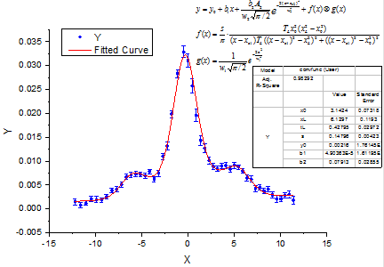
^2}{w_2^2}}+(f\;*\;g)(x)")
where =\frac{s}{\pi}\cdot\frac{\tau_Lx_0^2(x_L^2-x_0^2)}{(x-x_{c1})\tau_L((x-x_{c1})^2-x_L^2)^2+((x-x_{c1})^2-x_0^2)^2}") , ,
=\frac{1}{w_1\sqrt{\pi/2}}e^{-\frac{2x^2}{w_1^2}}") . .
And  , ,  , ,  , s, , s,  , ,  and and  are fitting parameters. are fitting parameters.  , ,  , ,  , ,  and and  are constants in the fitting function. are constants in the fitting function.
Read this tutorial for more details.
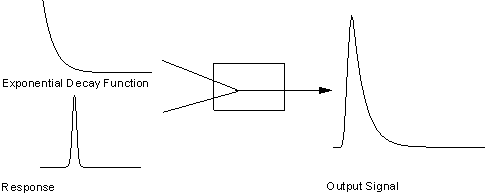
Convolution of Exponential Decay Function with Gaussian Response
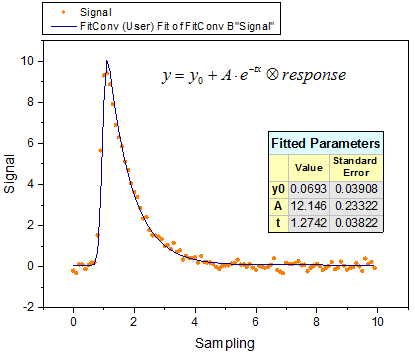
This experiment assumes that the output signal was the convolution of an exponential decay function with a Gaussian response as shown below:
Now that we already have the output signal and response data, we can get the exponential decay function by fitting the signal with the below model:

Read this tutorial for details.
If you need to deconvolute a peak, please refer to this Quick Help.
Fit Piecewise Function
Origin inherently provides two commonly used piecewise functions in Piecewise category:
- PWL2 -- piecewise linear function with two segments.
- PWL3 -- piecewise linear function with three segments.
If you need to create a new piecewise function, it would be necessary to read through the tutorials below:
Case 1
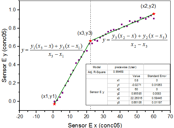
From the above graph, the curve consists of two segments of lines. It can be fitted with a piecewise linear function. The function can be expressed as:
+y_3(x-x_1)}{x_3-x_1}, & \mbox{if } x<x_3 \\
\frac{y_3(x_2-x)+y_2(x-x_3)}{x_2-x_3}, & \mbox{if } x \ge x_3
\end{cases}")
where x1 and x2 are x values of the curve's endpoints and they are fixed during fitting, x3 is the x value at the intersection of two segments, and y1, y2, y3 are y values at  respectively. respectively.
Read this tutorial to learn more details.
Case 2
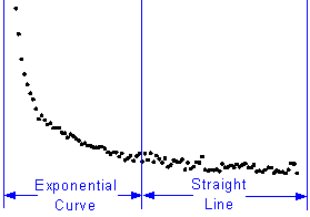
From the above graph, the curve consists of exponential curve segment and straight line segment as defined by equation below:

Read this tutorial to learn more details.
Fit with Multiple Variables
Origin inherently provides three commonly used multiple variables functions in Multiple Variables category:
- GaussianLorentz -- a combination of Gaussian and Lorentz functions with shared baseline and peak center.
- HillBurk -- a ombination of Hill and Burk models with two independent and two dependent variables.
- LineExp -- a combination of Line and Exponential models with one independent and two dependent variables.
If you need to create a new multiple variables function, it would be necessary to read through the tutorials below:
Fit a Curve with Two Different Functions Sharing Parameters
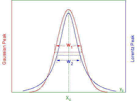
Fitting function for above graph is a combination of the Gaussian and Lorentz functions, sharing y0 and xc:
^2}{w_1^2}}")  ^2+w_2^2}")
Read this tutorial to learn more details.
Fit with Two Independent Variables
*x1}")
where x1, x2 are independent variables and ki, km, vm are fitting parameters.
Read this tutorial to learn more details.
Fit Complex Function
To fit a complex function in Origin, you need to separate the real and imaginary part of complex data into two different columns as two dependent variables.
Below is an example to show how to define your complex function:
complex cc = A/(1+1i*omega*tau);
	y1 = cc.m_re;
	y2 = cc.m_im;
where 1i is used as imaginary unit "i", omega is independent variable, A, tau are fitting parameters, y1 and y2 are the real and imaginary part of cc.
Fit with Ordinary Differential Equation
Origin allows you to define a first order or higher ordinary differential equation (ODE) by calling NAG functions.
Below is an example to show how to fit a first order ordinary differential equation:
 
where a is a parameter in the ordinary differential equation and y0 is the initial value for the ODE. NAG functions d02pvc and d02pcc are called using the Runge–Kutta method to solve the ODE problem.
Read this tutorial to learn more details.
Fit with External DLL
Origin C functions can make calls to functions in external DLLs created by C, C++, or Fortran compilers. To do this, your source file must contain an include directive for the header file which declares the functions in your external DLL.
Below is an example to show how to use GSL function from GNU Scientific Library to fit the following model:

Read this tutorial to learn more details.
If you want to know more about calling third party DLL functions, please refer to this page.
Quote Built-in Function in User Defined Fitting Function
Origin allows you to quote built-in function in defining a new fitting function.
Below is an example to show how to fit a skewed Gaussian peak, which can be considered as composed of two Gaussian functions. These two Gaussian curves share the same baseline and peak center (xc), but differ in peak width (w) and amplitude (A).
The function body is defined as:
y = x<xc? nlf_Gauss(x, y0, xc, w1, A1) : nlf_Gauss(x, y0, xc, w2, A2);
where nlf_Gauss() is the built-in Gauss function.
Read this tutorial to learn more details.
|