15.4 Interpreting Regression ResultsInterpret-Regression-Result
Regression is used frequently to calculate the line of best fit. If you perform a regression analysis, you will generate an analysis report sheet listing the regression results of the model. In this article, we explain how to interpret the imporant regressin reslts quickly and easily
In Parameters Table
The fitted values are reported in the Parameters table, like what is shown below:
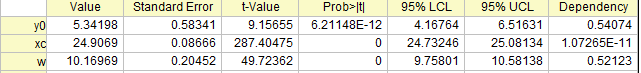
Value
Estimated values for each parameter of the best fit which would make the curve closest to the data points.
Standard Error
The parameter standard errors can give us an idea of the precision of the fitted values. Typically, the magnitude of the standard error values should be lower than the fitted values. If the standard error values are much greater than the fitted values, the fitting model may be overparameterized.
t-Value
Prob>|t|
Is every term in the regression model significant? Or does every predictor contribute to the response? The t-tests for coefficients answer these kinds of questions.
The null hypothesis for a parameter's t-test is that this parameter is equal to zero. So if the null hypothesis is not rejected, the corresponding predictor will be viewed as insignificant, which means that it has little to do with the response.
The t-test can also be used as a detection tool. For example, in polynomial regression, we can use it to determine the proper order of the polynomial model. We add higher order terms until a t-test for the newly-added term suggests that it is insignificant.
- t-Value: the test statistic for t-test
- t-Value = Fitted value/Standard Error, for example the t-Value for y0 is 5.34198/0.58341 = 9.15655.
- For this statistical t-value, it usually compares with a critical t-value of a given confident level
 (usually be 5%). If the t-value is larger than the critical t-value ( (usually be 5%). If the t-value is larger than the critical t-value ( ), it can be said that there is a significant difference. ), it can be said that there is a significant difference.
- However, the Prob>|t| is easier to interpret, and we recommend that you ignore t-Value and judge by Prob>|t|.
- Prob>|t|: The p-value for t-test
- If Prob>|t| < (usually be 5%), that means we find enough evidence to reject H0 of t-test. The smaller Prob>|t|, the more unlikely the parameter is equal to zero.
LCL and UCL (Parameter Confidence Interval)
UCL and LCL, upper and lower confidence intervals of parameter, indicate how likely the interval is to contain the true value. For example, in the above image of Parameters table, we are 95% sure that the true value of offset(y0) is between 4.16764 and 6.51631, the true values of center(x0) is between 24.73246 and 25.08134, and the true values of width(w) is between 9.75801 and 10.58138.
Dependency
The dependency value, which is computed from the variance-covariance matrix, typically indicates the significance of the parameter in your model. For example, if some dependency values are close to 1, this could mean that there is mutual dependency between those parameters. In other words, the function is over-parameterized and the parameter may be redundant. Note that you should include restrictions to make sure that the fitting model is meaningful, which you can refer to this section.
In Statistics Table
The key linear fit statistics are summarized in the Statistics table, like what is shown below:
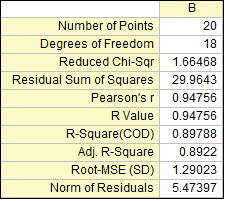
Residual Sum of Squares
Residual Sum of Squares is usually abbreviated to RSS. It is actually the sum of the square of the vertical deviations from each data point to the fitting regression line. It can be inferred that your data is perfect fit if the value of RSS is equal to zero. This statistic can help to decide if the fitted regression line is a good fit for your data. Generally speaking, the smaller the residual sum of squares, the better your model fits your data.
Scale Error with sqrt(Reduced Chi-Sqr)
The Reduced Chi-square value, which is also called Scale Error with square, is equal to the residual sum of square (RSS) divided by the degree of freedom. Typically a Reduced Chi-square value close to 1 indicates a good fit result, and it implies that the difference between observed data and fitted data is consistent with the error variance. If the error variance is over-estimated, the Reduced Chi-square value will be much less than 1. For under-estimated error variance, it will be much greater than 1. Note that it needs to select the correct variance in fitting procedure for Reduced Chi-square. For example, if the y data is multiplied by a scaling factor simply, the Reduced Chi-square will be scaled as well. Only if you also scale the error variance by a correct factor, the value of Reduced Chi-square will turn back into a normal value.
Pearson's r
Pearson’s correlation coefficient, denoted by Pearson’s r, can help to measure the strength of linear relationship between paired data. The value of Pearson’s r is constrained between -1 to 1. In linear regression, a positive value of Pearson’s r indicates that there is positive linear correlation between predictor variable(x) and response variable(y), while a negative value of Pearson’s r indicates that there is negative linear correlation between predictor variable(x) and response variable(y). The value of zero indicates that there is no linear correlation between data. What’s more, the closer the value is to -1 or 1, the stronger linear correlation is.
R-Square (COD)
R-square, which is also known as the coefficient of determination (COD), is a statistical measure to qualify the linear regression. It is a percentage of the response variable variation that explained by the fitted regression line, for example the R-square suggests that the model explains approximately more than 89% of the variability in the response variable. Hence, R-square is always between 0 and 1. If R-square is 0, it indicates that fitted line explains none of the variability of the response data around its mean; while if R-square is 1, it indicates that the fitted line explains all the variability of the response data around its mean. In general, the larger the R-square, the better the fitted line fits your data.
Adj. R-Square
R-square can be used to quantify how well a model fits the data, and R-square will always increase when a new predictor is added. It is a misunderstanding that a model with more predictors has a better fit. The Adj. R-square is a modified version of R-square, which is adjusted for the number of predictor in the fitted line. Thus, it can be used to compare with the fitted lines with different numbers of predictors. If the number of predictors is greater than 1, Adj.-square is always smaller than R-square.
In ANOVA Table
How the regression equation account for the variability in the ys is answered in ANOVA table, like what is shown below:
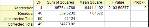
F Value
F Value is a ratio of two mean squares,which can be computed by dividing the mean square of fitted model by the mean square of error. For example, the F value of the model above is 65764.4768/16441.1192=2103.59577. It is a test statistic for a test of whether the fitted model differs significantly from the model y=constant, which is a flat line with slope being equal to zero. It can be inferred that the more this ratio deviates from 1, the stronger the evidence for the fitted model differing significantly from the model y=constant.
Prob>F
Prob>F is a p-value for F-test, which is a probability with a value ranging from 0 to 1. If the p-value for F-test is less than the significant level (usually be 5%), it can be conclude that the fitted model is significantly different from the model y=constant, which inferred that the fitted model is a nonlinear curve or a linear curve with slope that significantly different from zero.
| Notes: In linear regression, if fixing the intercept at a certain value, the p value for F-test is not meaningful, and it is different from that in linear regression without the intercept constraint.
|
In Covariance and Correlation Table
The relationship between the variables can be obsevered in Covariance and Correlation table, like what is shown below:
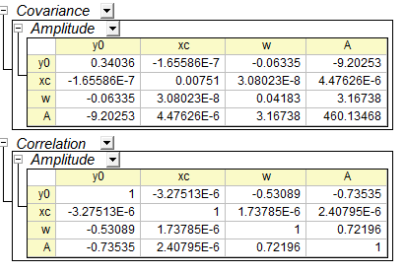
Covariance
The covariance value indicates the correlation between two variables, and the matrices of covariance in regression show the inter-correlations among all parameters. The diagonal values for covariance matrix is equal to the square of parameter error.
Correlation
The correlation matrix rescales the covariance values so that their range is from -1 to +1. A value close to +1 means the two parameters are positively correlated, while a value close to -1 indicates negative correlation. And a zero value indicates that the two parameters are totally independent.
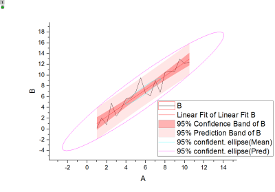
The fitted curve as well as its confidence band, prediction band and ellipse are plotted on the Fitted Curves Plot as below, which can help to interpret the regression model more intuitively.
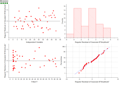
The residual is defined as:

Residual plots can be used to assess the quality of a regression, which is usually at the end of the report as below:
Topics for Further Reading
|