2.5.1.1 Tutorial for Parametric Distribution Analysis (Right Censoring)Tutorial-Parametric-Distribution-Analysis-Right-Censoring
In this example, a battery factory collected the battery lifetime from after-sales service data, defining lifetime as the elapsed time until capacity drops below 70 % (i.e., a 30 % loss). Using these right-censored data, engineers will run Parametric Distribution Analysis to obtain survival plots and key quantities (such as the ages at which 0.1 % and 99.9 % of batteries fail, and the proportions still running after 0.5, 1 and 1.5 years), providing the quantitative basis for future warranty policy.
 | Topics for Parametric Distribution Analysis for Right Censoring:
|
Sample Data
Right click on the Reliability and Survival app icon  and choose Show Sample Folder to open the sample project RSASample.opju. Go to sub-folder 1. Parametric Distribution Analysis (Right Censoring). and choose Show Sample Folder to open the sample project RSASample.opju. Go to sub-folder 1. Parametric Distribution Analysis (Right Censoring).
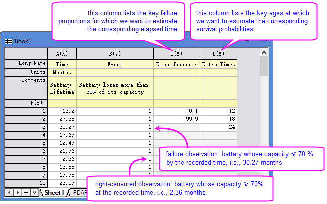
[Book1]Sheet1 shows a typical right-censored dataset.
- Each row represents one unit.
- "Time " column contains the exact failure time or the last recorded time if the unit is still working.
- "Event " column contains the censoring values: in this example, 0 = right-censored (unit still working at the record time); 1 = failure.
If your data contains multiple groups (e.g., different types or conditions), you can
- separate each group in its own time & censoring column pair, or
- stack all groups in one pair of time & censoring columns, and have a separate grouping column.
The tool will process each group in sequence, and export all results in a single report.
Steps
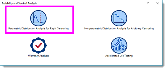
- With [Book2]Sheet1 active, click the Reliability and Survival app icon in the App Gallery . In the opened panel, choose Parametric Distribution Analysis for Right Censoring.
- In the dialog that opens, specify the settings as follow:
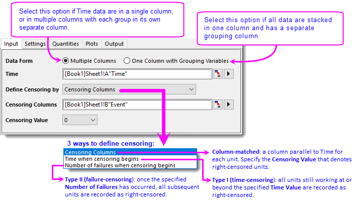
- On Input tab, select column A for Time. Make sure Define Censoring by is set to Censoring Columns and select column B for Censoring Columns. Origin will scan column B and populate the Censoring Value drop-down. Select 0 from it.
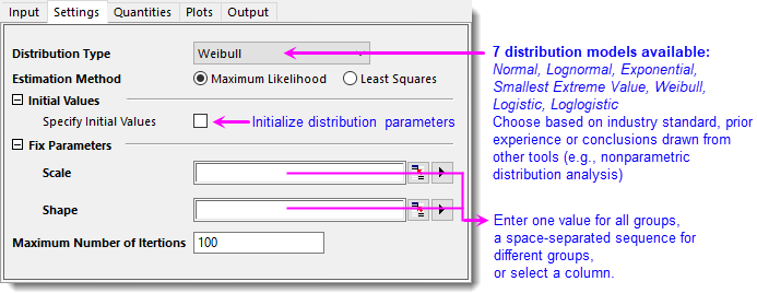
- On Settings tab, choose Weibull as Distribution Type. Estimation Method defaults to Maximum Likelihood. For more information about all 7 distributions and 2 estimation methods, refer to this page. Leave all other settings unchanged.
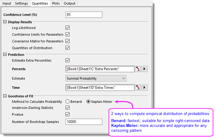
- On Quantities tab, expand Prediction branch. To estimate ellipse lifetimes at extra percentiles, check Estimate Extra Percentiles and then choose column C as Percents. To estimate survival percentiles at key moments, select Survival Probability for Estimate, and choose column D for Time.
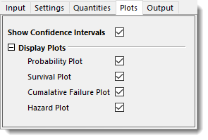
- On Plots tab, make sure all plots are checked.
- Click OK button to generate report sheets.
Results and Interpretation
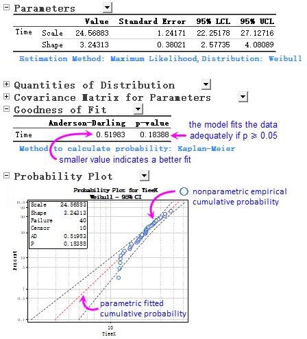
- The Parameters table reports the fitted Scale and Shape of Weibull distribution. All survival probabilities and plots derive from this model. We can examine the fit by the Goodness of Fit table and Probability plot below.
- Origin by default uses the Kaplan-Meier method to calculate the empirical distribution and outputs the Anderson-Darling statistic and p-value. p = 0.18388 > 0.05, indicates that the chosen model is acceptable.
- The P-P plot shows almost all points fall between 95% confidence bands, despite slight down warping in the tail, confirming the adequacy of the model.
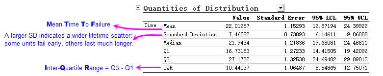
- The Quantities of Distribution table describes the fitted Weibull distribution characteristics by its centre and spread.
- Mean (MTTF) and Median locate the distribution centre.
- Median is the time by which 50 % of units have failed. Median = 21.943 months, indicates that 50 % of batteries have failed by this age.
- Mean is the arithmetic average of all failure times. Mean = 22.020 months, which is pulled higher by the right tail and therefore slightly larger than Median. Since Mean > Median (22.020 > 21.943), the distribution shows a mild right-skew: a tail of batteries that survives considerably longer than the typical lifetime.
- Standard Deviation and IQR measures the distribution spread.
- SD = 7.463 months, quantifies overall variability.
- IQR = Q3 – Q1, covers the middle of 50% population and is robust against extreme long-tail values. With IQR = 10.44 months vs. SD = 7.463 months, we can tell that the bulk of failures concentrates in a window of about 10 months with a moderate right tail.

- Refer to the PDARCPred worksheet for the estimated time at each failure rate (increasing by 1%). It also exports the times at the extra percents and the survival probabilities at the extra times we specified in Quantities tab. For example, 0.1% of batteries are estimated to fail by 2.92 months, and about 90.675% (0.90675) are still working after hours.
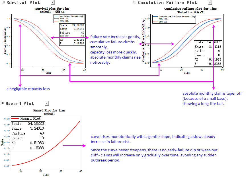
- Besides P-P plot, parametric distribution analysis exports the Survival Plot, Cumulative Failure Plot, and Hazard Plot, giving you an immediate visual overview of your data based on the chosen Weibull model.
|