2.5.2.1 Tutorial for Nonparametric Distribution Analysis (Arbitrary Censoring)Tutorial-Nonparametric-Distribution-Analysis-Arbitrary-Censoring
In this example, a factory has two types of high-lift pumps and want to investigate their service life. To control costs, engineers shut down, disassembled, and inspected the pumps every 1,000 hours, recording arbitrarily censored data up to 8500 hours. They will now use Nonparametric Distribution Analysis to obtain and compare the survival-probability plots of the two types.
 | Topics for Nonparametric Distribution Analysis for Arbitrary Censoring:
|
Sample Data
Right click on the Reliability and Survival app icon  and choose Show Sample Folder to open the sample project RSASample.opju. Go to sub-folder 2. Nonparametric Distribution Analysis (Arbitrary Censoring) . and choose Show Sample Folder to open the sample project RSASample.opju. Go to sub-folder 2. Nonparametric Distribution Analysis (Arbitrary Censoring) .
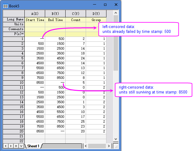
[Book2]Sheet1 shows a typical censored data for nonparametric distribution analysis - a combination of left-, right-, and interval censored observations. This example includes two groups, each group begins with a left-censored entry, continues with several interval censored entries, and end with a right-censored line.
Origin’s right-censoring analysis requires the censored data arranged in the following format:
- Start time: beginning of the interval (months, weeks, seasons, etc.),
- End time: end of the interval (same unit as Start time),
- Frequencies: count of failures in the interval.
- For left-censored units (1st and 11th row in this example), the Start Time is missing. Frequencies counts units already failed by the End Time
- For right-censored units (10th and20th row), the End Time is missing. Frequencies counts units still surviving at the Start Time.
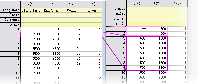
The Frequencies column is optional. If omitted, you can duplicate the interval and each duplicate represents one failure.
Note: If your data contain only exact failure times or right censored observations, please use Parametric Distribution Analysis for Right Censoring instead.
Steps
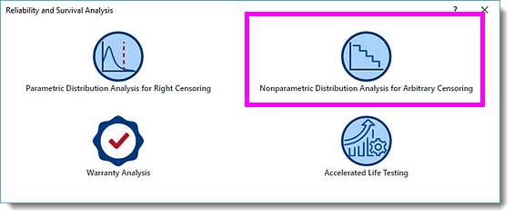
- With [Book2]Sheet1 active, click the Reliability and Survival app icon in the App Gallery . In the opened panel, choose Nonparametric Distribution Analysis for Arbitrary Censoring.
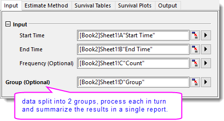
- In the dialog that opens, specify the settings as follow:
- On Input tab, select column A for Start Time, column B for End Time, column C for Frequency, and column D for Group, respectively.
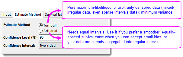
- On Estimate Method tab, Estimation Method uses Turnbull by default. For more information about the two estimation methods, refer to this page. Keep these settings unchanged.
-
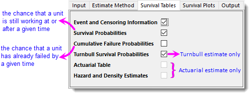
- On Survival Tables tab, check Turnbull Survival Probabilities checkbox.
-
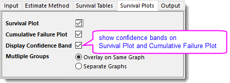
- On Survival Plots tab, select Cumulative Failure Plot and Display Confidence Band checkboxes.
-
- Click OK button to generate report sheets.
Results and Interpretation
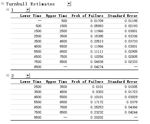
- The Turnbull Estimates table reports the failure timing. We can see that for type 1, the failure peak, 20.513% (0.20513), failed between 3500-4500 hours, while for type 2, the failures peak happened in two intervals, 25.253% (0.25253) in 6800-7500 h and 23.232% (0.23232) in 7500-8500 h. Peak of type 2 shifted more than 3000 h later.
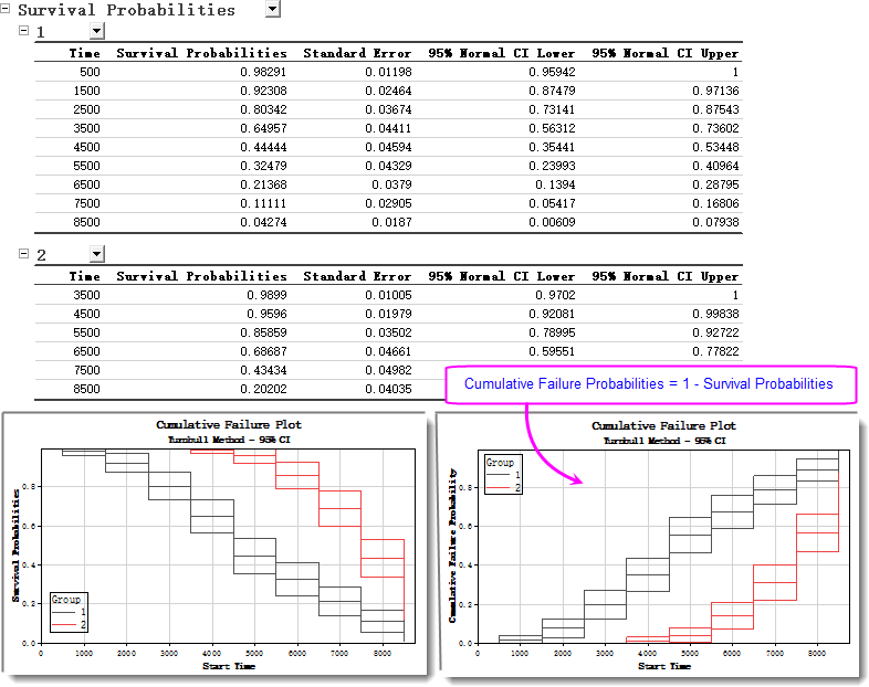
- The Survival Probabilities table gives the probability that a unit is still working at each specific time point and is used to check reliability requirement. From it we can tell that in the confidence interval of 95%, the pumps of type 1 can be used about 500 hours but drops below 95% soon after, whereas type 2 remains until at least 4500 h. This order-of-magnitude difference, which is also visible in both the Survival Analysis Plots and Cumulative Failure Plots, confirms that type 2 pumps are significantly more reliable than type 1.
From this report we can conclud that without a specific parametric distribution assumption, pumps of type 2 demonstrate significantly higher reliability. Engineers should focus on improvements in materials and processes for type 2 to push failures even further out.
|