2.5.4.1 Tutorial for Accelerated Life Testing

Tutorial-Accelerated-Life-Testing

In this example, an electric vehicle factory wants to test the battery lifetime (capacity drops below 70 %). Tracking this under normal conditions can take years and is both time-consuming and costly. To compress the timeline to several months, the engineers accelerate wear-and-tear by elevated temperatures (40, 60 and 80 °C), record the failures every month, and then use Accelerated Life Testing to predict lifetimes at normal operating temperature (30 and 50 °C).

Topics for Warranty Analysis: Algorithm

Sample Data

Right click on the Reliability and Survival app icon and choose Show Sample Folder to open the sample project RSASample.opju. Go to sub-folder 4. Accelerated Life Testing .

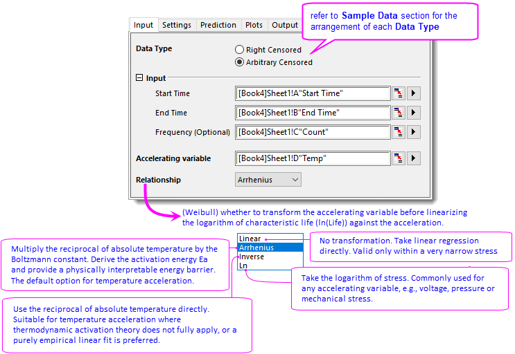
ALT tool supports two types of data arrangement.

• Arbitrary Censored
  [Book4]Sheet1 shows an example of arbitrary censored dataset for ALT - a mixture of right- and interval-censored observations. The censored data is arranged in the following format:
  • Start time (column A): beginning of the interval (months, weeks, seasons, etc.).
  • End time (column B): end of the interval (same unit as Start time). If Start time = End time, the unit failed at the exact time.
  • Frequencies (column C): count of failures in the interval. Optional. See below for details.
  • For left-censored units, the Start Time is missing. Frequencies counts units already failed by the End Time
  • For right-censored units (7th, 14th and 21st rows), the End Time is missing. Frequencies counts units still surviving at the Start Time.
  • Accelerating variable (column D): corresponding stress level for each unit.

  

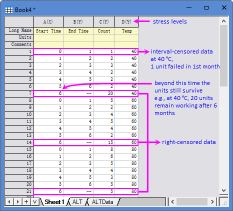
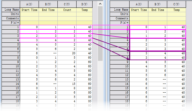
  The "Frequencies" column is optional. If omitted, you can duplicate the interval and each duplicate represents one failure.

  

• Right Censored
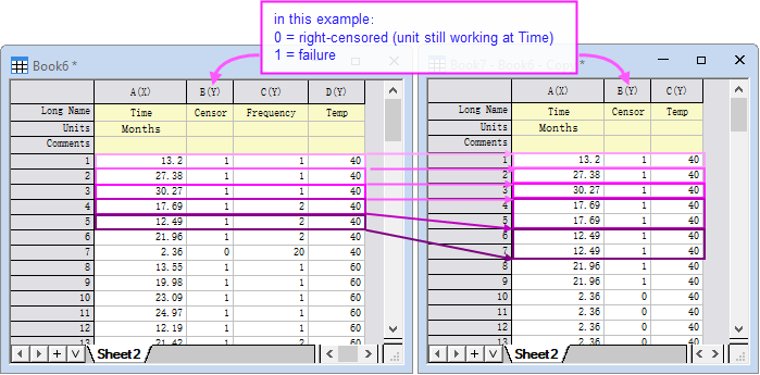
  The right-censored data is arranged in the following format:
  • "Time " (column A): the failure time or the last recorded time if the unit is still working (right-censored).
  • "Censor " (column B): the censoring values.
  • Frequencies (column C in the left): count of units. Optional. If the "Frequencies" column is omitted, you can duplicate the entry and each duplicate represents one unit.
  • Accelerating variable (column D in the left/column C in the right): corresponding stress level for each unit.

  

Steps

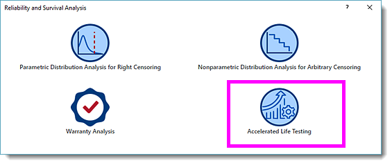
1. With [Book4]Sheet1 active, click the Reliability and Survival app icon in the App Gallery . In the opened panel, choose Accelerated Life Testing.

   

2. In the dialog that opens, specify the settings as follow:
   • On Input tab, select Arbitrary Censored for Data Type. Choose column A for Start Time, column B for End Time, column C for Frequency, and column D for Accelerating variable, respectively. Since the accelerating variable is temperature in this example, select Arrhenius from Relationship dropdown list. Refer to this page for details of relationship.

     

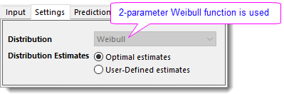
   • On Settings tab, Distribution is set to Weibull and Distribution Estimates to Optimal estimates by default. Keep these settings unchanged.

     

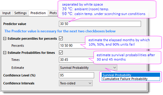
   • On Prediction tab, type 30 50 in Prediction value edit box to extrapolate lifetime at these two temperatures. Check Estimate percentitles for percents checkbox, and type percentiles 10 50 90 in Percents edit box. Check Estimate Probabilities for times, type 30 45 in Time edit box and select Survival Probability for Estimate.

     

   • On Plots tab, under Display Plots branch, check Probability Plot for each accelerating level by fitted model, and enter 30 to Design value to include on plots edit box. Check Relation Plot and enter 10 50 90 to Percents edit box. Check Probability Plot for each accelerating level by individual fit.

     

3. Click OK button to generate report sheets.

Results and Interpretation

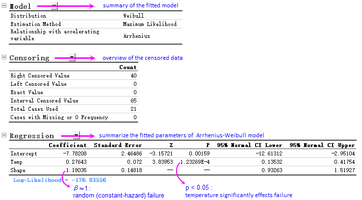
• The Regression table reports the key parameters of the fitted Arrhenius-Weibull model.
  • Intercept -7.782 and Temp 0.276 (slope) versus the transformed temperature determine the characteristic life at any design temperature. Refer to this page for equations and detailed algorithm.
  • Shape of the Weibull distribution (calculated by MLE) help you understand the failure mode.
  • The activation energy and acceleration factor are also derived from Temp, understand how strongly temperature accelerates the failure.

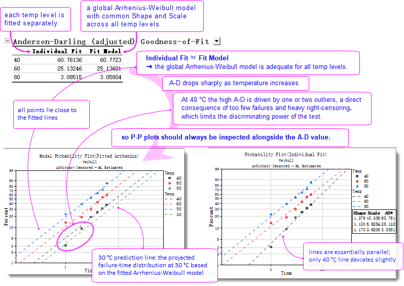
• Origin calculates the difference between the empirical distribution (by Kaplan-Meier) and fitted distribution, and outputs the Anderson-Darling statistics for individual fit under each temperature ("Individual Fit" column) and overall model of all temperatures ("Fit Model" column).
• The near-equal A-D values for individual and global fits show that a single Arrhenius-Weibull model is good enough for all temperature levels.
• A-D statistics provide a quantitative gauge of the fit: smaller value indicates a better fit; but the final conclusion should always come from the Probability Plot.
• The Model Probability Plot (global model) shows that almost all points lie close to the fitted line, despite slight down warping in the tail of 40 °C (yet it remains in the 95% confidence interval if you choose to turn on CI on the Plots tab of the dialog). The Probability Plot (Individual Fit) gives the same picture: 60 °C and 80 °C lines are essentially parallel, while 40 °C line shows a small angle. Both P-P plots confirm the adequacy of the global Arrhenius-Weibull model across the accelerating temperatures, with only minor bias at lower temperature.
• A 30 °C reference line is superimposed on the Model P-P plot to display the predicted cumulative failure probabilities under the use-condition temperature, providing a direct benchmark for future validation data and warranty policy.

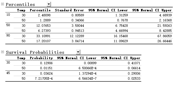
• The Percentiles table estimates the elapsed months at which the specified percentages of batteries will fail, and the Survival Probabilities table gives the probability that a unit is still working at each specified time point. Both can be used to verify reliability requirements. For example, at 30 °C, 10% of batteries will fail by 2.48 months and 90% by 33.11 months. After 30 months (about 2.5 years) about 12.9% of batteries can still work at 30 °C, whereas at 50 °C the survival probability fails below 1.2% - an order-of-magnitude drop indicates how rapidly battery capacity is lost as temperature increases.

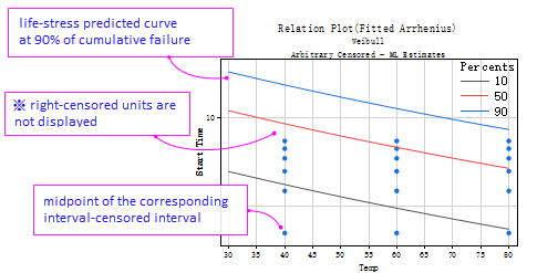
• Relation plot shows the percentile lines (the 10%, 50%, and 90% in this example) predicted by Arrhenius-Weibull model described in Regression table, and is used to assess the relationship of lifetime (or ln(life)) and the accelerating stress. Censoring data (exact failure time and interval censored) are added on the plot for visual comparison.
• If a large proportion of the observations is censored, just like this example, all data are interval-censored or right-censored data, the Relation plot cannot be trusted to validate the relationship assumption. Instead, Anderson-Darling statistics and P-P plot should be used for a decision.