4.3.6 Displaying Supporting Data in Worksheet Header Rows

WksHeaderRow-DataSupportDisplay

Origin worksheet supports header rows above data area for metadata. Such metadata in these header rows then becomes available for plotting and analysis operations. By default, the workbook template that ships with Origin only shows the Long Name, Units, Comments and F(x) row headings. User can turn on extra header rows during import, such as sampling interval, sparklines, etc.

User can also manually add extra user-defined or built-in parameters rows. Note, only info. in user-defined or built-in parameter rows can be formatted, e.g. set as numeric with certain decimal places showing, set as Date or Time, etc.

Also, be sure to see Simple Utilities for Filling Columns with Data.

Display Column Label Rows

By default, the Origin worksheet template displays four column label rows -- Long Name, Units, Comments and F(x)= (column formula). These column label rows can be added to or hidden depending on your need to display supporting information in the worksheet.

There are several ways to control label row:

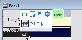
1. Use mini toolbar. Column label row mini toolbar is introduced in recent versions. Single click on a row label row header or multiple row headers will see mini toolbar. Hide, move up and Move down selected row(s), click P button there to add user-defined paramater row.
2. Use context menu. Right click on a column label row header or multiple row headers to show/hide, set as Long Name, Unit, or add user-defined parameter, etc.

   

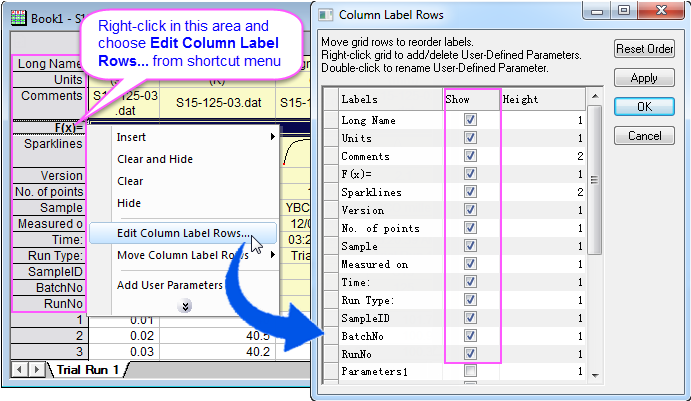
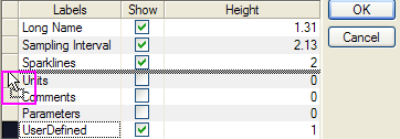
3. Use Column Labe Rows dialog. Right-click on any column label row header and choose Edit Column Label Rows... context menu. Turn on/off header rows, drag to reorder label rows, create, rename or delete UserDefined parameters, delete.

   

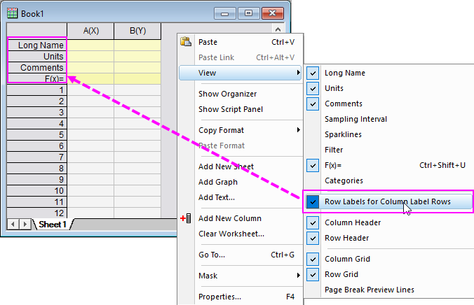
4. Use View: context menu. Right-clicking on (a) the window's title bar or (b) the empty space to the right of the worksheet columns (but inside the workbook window) and choose View from the shortcut menu (see the picture below) and uncheck your row heading display selections.

   

Set Styles

Use Mini toolbar or Worksheet Properties dialog to set column label rows styles or use context menu to set styles.

• check RTF(Rich Text) checkbox to display greek letter, LaTeX or special characters.
• Check Wrap Text to wrap long text.
• Choose Open Properties dialog button/Set Style -> More... context menu to go to go to the format tab of worksheet properties dialog for further customization, such as float text into next cell, dynamic merge, etc.

Note: If Rich Text isn't checked, greek letters, special characters and LaTeX can only show as escape sequences in worksheet, e.g. \g( ) for Greek text, \q( ) for LaTeX, etc. though they will show fine in graph such as axis title, legend, etc.

Copy and Paste Column Label Rows

To copy all column label row(s), right click the column Label Row to copy (Edit: Copy or Ctrl+C) and then go to destination to paste (Edit: Paste or Ctrl+V). Paste Transpose, Paste-link are also supported.

To copy selected column(s) label row metadata together with column(s) data, right-click column(s) and choose Copy (including label rows). Non-contiguous selections and worksheet subrange selections are supported.

• To paste only label row values, right-click on the cell in the upper-left corner of the label row area and Paste (Origin will not add User Parameter rows).
  
• To paste only data row values, right-click on the cell in the upper-left corner of the data area and Paste (Origin will add data rows, as needed).
  
• To paste both label and data values, select the left-most column by clicking on the column heading and Paste. Both metadata and data will be pasted to the worksheet. Columns, data rows and User Parameter rows will be added, as needed.

To copy selected column(s) label row metadata only, right-click column(s) and choose Copy (formula), Copy (label rows) or Copy (formula and label rows).

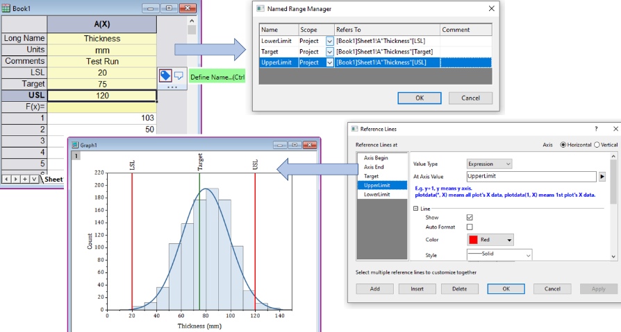
Define Named Range in Label Row Cell

You can define any column label row cell as a named range for use in such things as column formulas or reference lines.

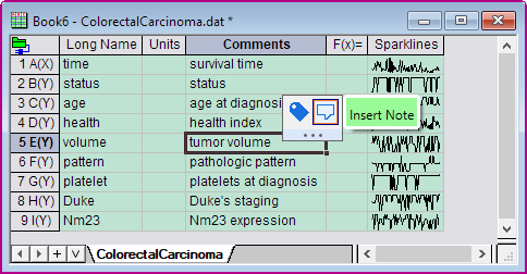
Inserting Notes to Label Row Cells

You can insert a popup note to any label row cell. For instance, adding a popup note to a Comments cell allows you to add extensive comments without having to use vertical space to display comments in full.

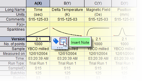
1. Click on the header row cell.
2. Click the Mini Toolbar button Insert Note.

• Notes support Origin Rich Text and can include such things as hyperlinks, tables, LaTeX equations and images.
• Notes content can be modified using Format toolbar buttons and/or a customizable set of Paragraph Styles.
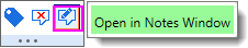
• Once a cell note is added, the user can reselect the cell, click the Open in Notes Window button and add and format elements.

• Popup notes display when the user hovers on the note tab in the upper-right corner of the cell.
• Popup notes are best-suited to display of simple text. Complex notes of mixed elements are best edited and viewed directly in the Notes window as opposed to the popup display.
• In Column List View, it also supports cell notes for column label row.

You can add Notes content to a graph or layout page using a "@@@NotesN" syntax.

Built-in Label Rows

Long Name

Column's short name is auto-named alphabetically and not changeable by default. So we recommend using column's Long Name row to put descriptive names.

For information on the worksheet column Long Name, see Origin worksheet column naming conventions.

Origin can make use of this information to annotate graphs. For instance, if the Long Name and Units are specified, they can be used to automatically label the X and Y axes of a 2D graph.

Units

The Units row stores the units for the worksheet data columns. Rich Text is on by default for Units row.

Another possible use for the Long Name and Units information is in the graph legend.

If after import, Units are appended to Long Name, (1) select the Long Name label row and (2) on the Mini Toolbar that appears, click the Extract Units from Long Name... button . If you prefer to leave Units appended to Long Name while also copying Units to the Units label row, clear the Remove from source box.

Comments

Each worksheet column can have one or more lines of Comments. Multiple comment lines can be typed into the Comments cell by pressing CTRL + ENTER at the end of each line. If you are importing files in which you've pre-defined multiple lines of comments, these are preserved and placed in the Comments cell.

F(x)

The F(x)= header row displays either:

• The column formula. This is a mathematical expression that is typically used to fill the column with values.
• The Formula Text. This is alternate text that can be typed directly into the cell or entered into the Formula Text dialog box to display in place of the column formula. For instance, when displaying a long formula in the cell is not practical, enable display of the Formula Text and display some meaningful indicator of the purpose of the column formula.

Direct editing of the cell can be turned on (default) or off. To turn off direct editing of F(x)=:

1. Open Set Values (with the column selected, choose Column: Set Column Values).
2. Click the Options menu.
3. Clear the check mark next to Direct Edit Formula Cell.

For help with creating column formulas, see Set Values, Quick Start and Set Values, Options Menu.

Use the Hotkey CTRL + SHIFT + U to show/hide the F(x)= row. You also can hide/show this row using corresponding shortcut menus, see this section. The default Recalculation Mode of F(x)= is Auto. One can change it by system variable @AUFL.

Creating the F(x)= expression

Expressions are entered into the F(x)= cell in one of three ways:

• Double-click on the cell and type an expression directly into the cell (assumes direct-edit is not disabled, as discussed in the previous section).
• Enter an expression in the upper panel of the Set Values dialog box.
• Enter an expression using a shortcut menu command (see next section).

You can disable autocompletion for column and/or cell formulas/F(x)=: Click Preferences: System Variables. In an empty Variable cell, type FAC. Enter one of the following in the Value cell (values are additive): 0 = turn off autocomplete, 1 = enable for cell formula and the F(x)= label row, 2 = enable for column formula, 3 (default) = enable for cell formula/F(x)= and column formula. Click OK to close the dialog.

To autofill formula containing column ShortName with shift, press Ctrl key while dragging the bottom-right corner of the formula cell. See this FAQ for more autofill methods.

F(x)= shortcut menu commands

Assuming direct editing is enabled, you can right-click on the F(x) cell, and enter information into the cell using one of the following:

You can also load formulas directly in the column label row F(x)= cell by selecting the cell and choosing Column: Fill with User Formula from the main menu.

F(x)= shortcut menu commands for Python function calls

When the column formula calls a Python function, an additional Open Python File shortcut menu command is shown, if:

• The F(x)= cell formula begins with py..
• The Python function is saved to an external file. By default that file is named labtalk.py and is saved to your User Files Folder. See documentation for the LabTalk Python object for information on current working directory and working file).

Selecting an F(x)= cell that meets the above criteria will show the path to the current working directory and file, on the Status Bar.

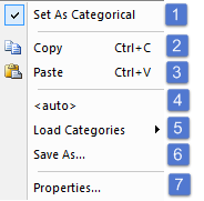
Categories

The Categories column label row displays when you have designated the worksheet column as containing categorical data (select the column, right-click and choose Set as Categorical ). The cell contents will show (a) whether data are sorted or unsorted (<auto> is selected) or (b) a space-separated list of categories:

• If you double-click this cell, you open the Categories dialog box (same as the Column Properties, Categories tab), with controls for display of the categorical data in this column.
• If you right-click this cell, you open a "categorical" shortcut menu that duplicates some key Categories tab controls.

1. Set or clear column as categorical
2. Copy categories (includes setting the column as categorical)
3. Paste categories (includes setting the column as categorical)
4. Set as <auto> (displays sorting info, dynamically generates categories from list) or display space-separated categories (not dynamically updated)
5. Load previously saved categories (default path is \User Files\Categories\)
6. Save categories to file
7. Choose Properties to open the Categories dialog box

For information on creating and customizing graph legends for plots of categorical data, see Legends for Categorical Data.

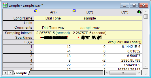
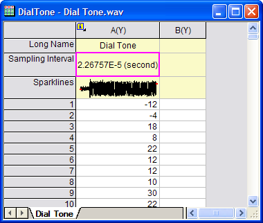
Sampling Interval

In an effort to reduce file size, some data files -- particularly those consisting of data collected at regular intervals -- may exclude the independent variable (X column). When this is the case, the Sampling Interval row will display the sampling (X) interval. You can see a quick demonstration of how this works by dragging and dropping a .WAV file into the Origin workspace.

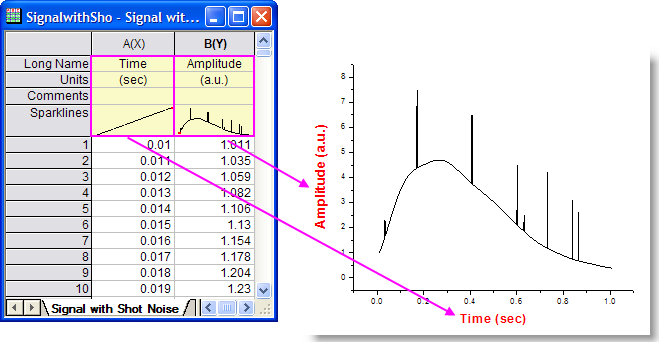
Sparklines

Sparklines can provide a quick view of trends in a set of related datasets contained in the Y columns in a worksheet.

To show sparklines in the worksheet:

1. From the main menu, choose Column: Add or Update Sparklines.
2. In the small dialog that opens, configure your sparklines.
3. Click OK to add them to the Sparklines label row.

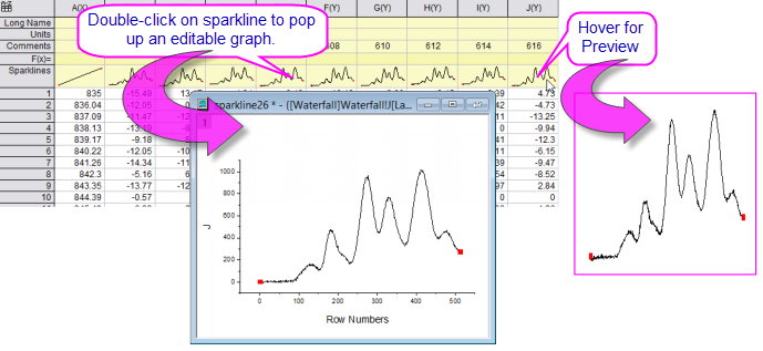
Note that each sparkline is an editable embedded graph which can be opened by double-clicking on the sparkline object (see the picture below) above each column of worksheet data. Additions to the graph are stored -- though not necessarily displayed -- in the embedded object. Hovering on a sparkline shows an enlarged view of the sparkline.

Sparklines can, in large numbers, cause Origin to act sluggishly. If your project is difficult to work with and you suspect sparklines may be contributing, you can prevent sparkline creation and hide existing sparklines in the project using system variable @SPK. Additionally, you can delete sparklines from the current project using delete -spk.

Filters

This row will show only when filter is added in any of the columns in worksheet. It shows the filter condition.

Parameters

The built-in Parameters rows are off by default but can be turned on to display extra information such as temperature, pressure, humidity, wavelength, etc. but since these built-in parameters cannot be renamed, most will find the UserDefined parameters to be more useful.

For an example of how worksheet Parameter information might be incorporated into an Origin graph, see Customizing Waterfall Plots.

To manually add a single parameter to the worksheet:

1. Right-click on any column label row to select Edit Column Label Rows... from context menu to open the Column Label Rows dialog box.
2. Check the Show check box for the label Parameter#, click OK button to add the parameter into the worksheet as a column label row.
3. Double-click on the parameter row heading you just added to open the Move to User Parameter dialog to change the parameter name and set it as a User Parameter.

User-Defined Parameters

You can add any number of user-defined parameter rows and assign any name to them.

To add a user-defined parameter row to the worksheet header:

• Click on any label row header and click P button on mini toolbar to insert before the selected row.
• Right click on any label row header and choose Add User Parameters... to add after the selected row.
• Right click on any label row header and choose Insert: User Parameter to insert before the selected row.
• Right click on any label row header and choose Edit Column Label Rows... to open the Column Label Rows dialog box.
  • Right click in the dialog to add and double click to rename.

  

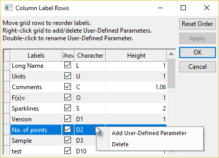
  • Drag the empty grid cell on the left to reorder.

  

  • The Character column lists the character used to refer to that column label row. Refer to this LabTalk document for details of how to access to column label rows.
  • You can select multiple rows (Ctrl+click to select contiguous rows or Ctrl + Shift + click to select discontiguous rows) to delete them at once. Note that built-in label rows cannot be deleted. So if the selection includes any built-in labels, those rows will be skipped.
• Activate the worksheet and select menu Format: Worksheet.... On View tab, click Edit Column Label Rows... button.

Note that user-defined parameter rows can also be created on data import, provided your data files contain metadata in the header and you have pre-defined parameters using the Import Wizard.

To move the contents of a built-in label row (e.g. Comments) to a user-defined parameter row:

• Double-click on the built-in row heading; or
• Right-click and choose Set As User Parameter.

These actions open a Move to User Parameter Row box where you can enter the name of your user-defined parameter and move the row content to the user-defined parameter row.

To rename a user-defined parameter:

• double-click on the parameter row heading and enter a name in the Name box of the opened Edit dialog. In this dialog, you can enable and enter a Formula for the user parameter for the purpose of calculating some column statistic, such as mean or standard deviation.

To hide/show all user parameters:

Data files generated from equipment may contains many meta data, which will be imported into user parameter rows. If there are too many user parameter rows, more than 10 rows for example, it is hard to scroll down to see the data area. In this case, you will need to hide the user parameter rows:

• Click on any label row, in the mini toolbar that pops up, select Hide/Show All User Parameters button .

To view all user parameters that have been hidden:

• Click on any built-in label row (LongName, Unit, or Comment), in the mini toolbar that pops up, select Hide/Show All User Parameters button ,
  or,
• In the Script Window, run LabTalk command:

wks.labels(D*)

Formatting User Parameters Data

All worksheet column label row data are stored as strings, even data that appear to be numeric. User Parameter rows do support the formatting of data that have the appearance of being numeric (e.g. a Julian date value such as "2458395").

• Click a user-defined parameter row and click the Open Properties dialog... button on the mini toolbar.
• Right-click on a row heading and choose Set User-Defined Style: More from the shortcut menu

Both open the Format Cells dialog box to set Format and Display.

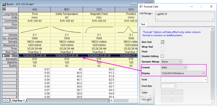
• More Custom Display formats are provided according to the data type you choose from the Format Cells dialog's Format drop-down list (Text & Numeric, Date or Time).
• You can apply formatting to Date and Time data only if the string stored in the user-defined parameter row is in numeric form (i.e. a Julian Date value as used internally by Origin). Formatting such numeric strings will also allow you to use these column label row values for calculation purposes such as in a worksheet cell formula (e.g. =value(wcol(j)[D1]$)).
• The user should always remember that despite whatever formatting options are applied, column label row data are still string data -- not numeric data.

Define a Formula when you Add User Parameters

You can add a user-parameter row to the worksheet expressly for the purpose of calculating some column statistic, such as mean or standard deviation.

1. Right-click on the column label row headings and choose Add User Parameters from the shortcut menu.
2. In the Add User Parameters dialog that opens, enter a name for your user-defined row, then click the flyout menu to pick from a list of common statistics. The statistic will be calculated for each data-containing column in the worksheet.

   

3. To make changes to a User Parameter row Name or Formula, right-click on the User Parameter row heading and choose Edit from the shortcut menu.

The above procedure automatically extends your formula across all worksheet columns. However, you can also extend a label row formula to all cells to the right of the formula-containing cell by hovering in the lower-right corner of the formula cell and double-clicking on the "+" icon.

If you want to apply a user-parameter row to other worksheets, especially those defined by formula,

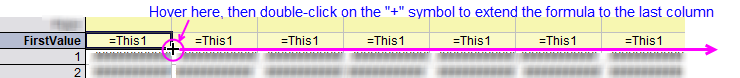
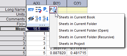
1. Select the user-parameter row you want to copy.
2. In the mini toolbar that pops up, select Apply User Parameters to button . In the fly-out menu, select the target worksheets:

• Sheets in Current Book: All sheets in current workbook. Hidden sheets will be included while embedded sheets will not.
• Sheets in Current Folder: All sheets in current folder. Sheets in subfolders will not be included. Hidden sheets will be included, while embedded sheets will not.
• Sheets in Current Folder (Open): All the opened (not hidden) sheets in current folder. Sheets in subfolders will not be included.
• Sheets in Current Folder (Recursive): All sheets in current folder. The subfolders will be recursively included.
• Sheets in Project: All sheets in the project. Hidden sheets will be included while embedded sheets will not.

Explanation of Context Menus for Column Label Rows

The following explains each context menu of column label rows.

Insert User Parameters

Select Insert:User Parameters from the right-click menu to insert a User Parameter above current column label row.

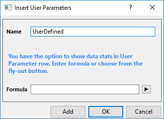
This dialog is same as the dialog "Add User Parameters".

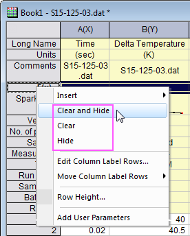
Hide/Show Column Label Rows

To hide one or more rows, you can right-click on column label row to select Hide or Clear and Hide from the context menu. If you select Clear and Hide, the information in the current label row will be cleared up and the entire row will be hidden.

To show the hidden column label rows, you can do selections from the View shortcut menu or go to the Column Label Rows dialog. See the details in this section.

Rename Row Label

The default displayed column label rows, Long Name, Units, Comments and F(x)= are not able to be renamed, also the Parameter row. Double-click on their row heading(right-click on the heading to select the Edit... context menu), the Move to User Parameter dialog will pop up to let you rename the row label, but convert it into a user parameter.

To rename the row label for an existing user parameter:

1. Double-click on the row heading to open the Edit dialog.
2. Enter a new name in the Name box, enable and enter a formula in the Formula box if needed.
3. Click OK to close the dialog.

Edit Customize Label Rows

Right click on the column label row and select Edit Column Label Rows... from the context menu, it will open the Column Label Rows dialog. In this dialog, you can hide/show a column label, reorder label rows, add a user-defined parameter, and specify the height for each label row.

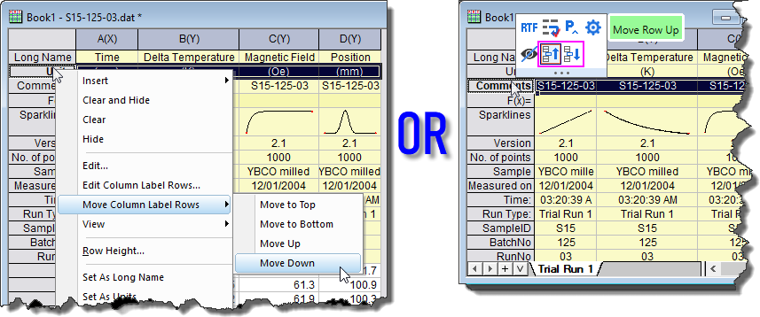
Move Column Label Rows

To move column label rows:

1. Right click on the column label row, select Move Column Label Rows, then select Move to Top/to Button/Up/Down in context menu.

Or,

1. Click on the column label row, click or button from mini toolbar.

Set Other Rows as Label Rows

To set one or more rows (column label rows or data rows) as three of the standard column headings (Long Name, Short Name and Units), user-defined parameters, right-click and select Set As Long Name/Units/Comment/User Parameters from the context menu.

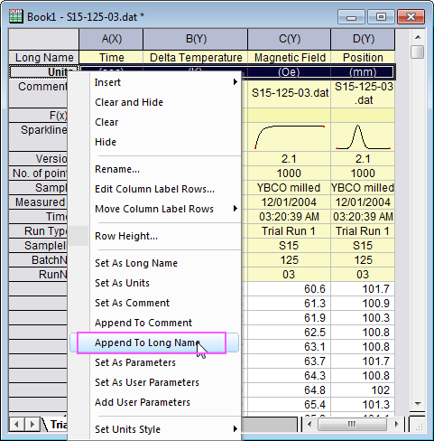
Append Rows to Label Rows

To append one or more rows to column Long Name or Comment:

1. Right-click on one or more rows (column label rows or data rows), select Append To Comment/Long Name from the context menu.

   

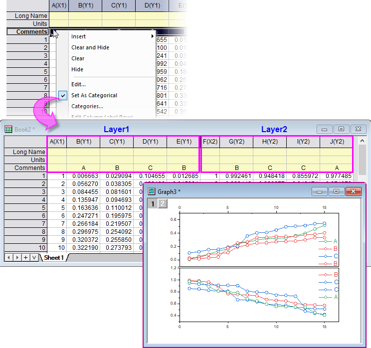
Set As Categorical

• Right click on a column label row and select Set As Categorical context menu.
  Or, select a column label row and click Categorical button from mini toolbar that appears.
  This will design the selected label row as containing categorical data.
• Available label rows including Long Name, Units, Comments, Parameters, and User Defined Parameters.
• Once a column label row is set as categorical, you can right click on it and select Categories context menu. This will open the Categories dialog, allowing you to customize categories.
• This feature is useful when you plot columns into multiple plot groups or layers, and for columns with same laabel row, you want to share the same plot properties (color, symbol shape, size, .etc) between different groups/layers. In this case, you can set this column label row as categorical and map plot color/shape/size... to this label row.