4.4.18 Pivot TableWks-Pivot-Table
A pivot table is a data summary tool commonly found in data-analysis software. The table is constructed by taking a dataset consisting of observations collected across a number of variables, picking two categorical variables of interest -- let's call them var1 and var2 -- then letting all possible values of var1 define rows in the table, and all possible values of var2 define columns in the table. Table cells would then contain values that result from the intersection of row and column values. A parallel of pivot table is a matrix, with the var1 as rows, var2 as columns, pivot table data as the elements of the matrix. By saving an analysis template with pivot table, you can quickly create similar data summary for different dataset.
Origin's pivot table tool includes support for the following:
- Summarize data by counts, or report a sum, a mean or min/max values.
- Provide totals on rows and columns.
- Sort output rows and columns by row totals or labels.
- Normalize by fractions or percentages.
- Combine smaller values into an "other" column.
- Adjust parameters and instantly recalculate.
To open this tool:
- Click on the worksheet that you want to analyze.
- Click Restructure: Pivot Table... to open the wpivot dialog box.
The wpivot dialog uses the the wpivot X-Function.
Dialog Options
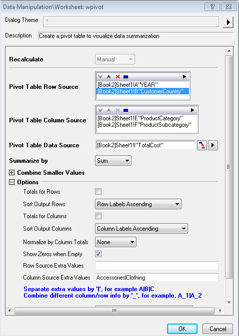
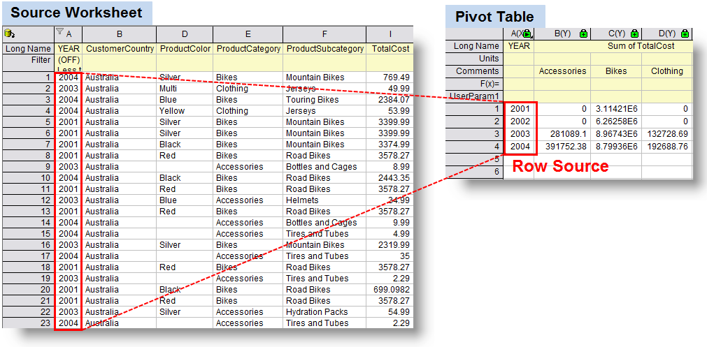
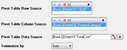
Pivot Table Row Source
Specify the column range that will be used as the row source of the pivot table. Data in the source worksheet with the same name in row source range will be displayed as a single row in the pivot table.The following diagram illustrates the definition of row source. You can choose one or more data range as pivot table row source.
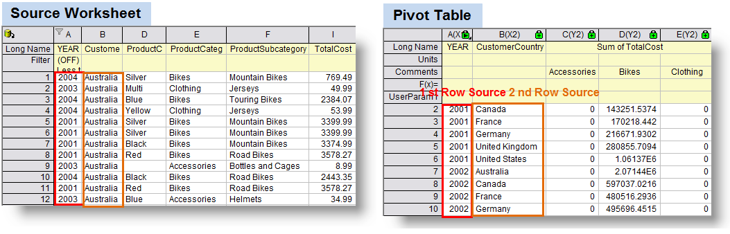
The following diagram illustrate the definition of multiple row source in pivot table.
This part includes a display box and a toolbar with five buttons  : :
| Display Box
|
The selected column(s) will display in this box. To do this analysis, you must select at least 1 column for the row source.
|
Triangle Button for Select 
|
Click this button then choose a column from menu, or click Select Columns to open the Column Browser and add column(s) to the Display Box as row source of pivot table. Click this button again to add another column as additional row source.
|
Remove button 
|
Remove the selected data range(s) from the Display Box. This button is available when you select one or more selected column(s) in the box.
|
Move Up button 
|
Move the selected data range(s) up in the Display Box. Use this button to order the row source columns and the pivot table results will follow this order.
|
Move Down button 
|
Move the selected data range(s) down in the Display Box. Use this button to order the row source columns and the pivot table results will follow this order.
|
Select All button 
|
Select all data range(s) down in the Display Box.
|
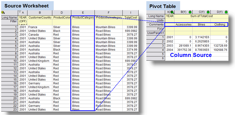
Pivot Table Column Source
Specify the column range that will be used as the column source of the pivot table. Data in the source worksheet with the same name in column source range will be displayed as a single row in the pivot table. The following diagram illustrate the definition of column source. It should be noted that the column information can be designated into other column label rows. You can choose one or more data range as pivot table column source. The column source arrangement in the pivot table would be similar to those of row source.
Note:
- This part includes a display box and a toolbar with five buttons .To know more about the controls, please refer to the table under the Pivot Table Row Source section.
- The value of Column Source has been put into the Comments column label row by default; in fact, it can be also put into other column label rows, such as Long Name by configuring the Put Column Info. to drop-down list of Options.
|
Pivot Table Data Source
This is available only when Count is not selected for Summarize by (the Method variable). These are the data values to be summarized from one dimension column into two dimension matrix-like pivot table.
- Summarize Data by Max, Min, Mean, or Sum
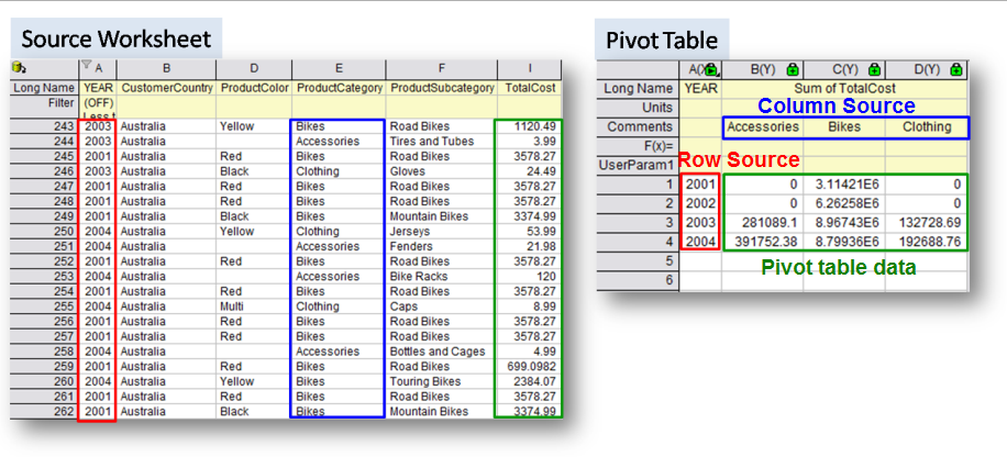
- The way data arranged in pivot table is similar when summarizing data by Max Min, Mean or Sum. The following screenshot is an example to summarize data by Sum
- In the following example, the total cost data of cell (2001, Bikes) is the sum of those cells in Column TotalCost with criteria as follow: ProductCategory as Bikes, and YEAR as 2001.
- On the contrary, if Count is selected in the Summarized by drop-down list, the table would only fill in the count number that simultaneously meeting its cell position that related row resource and column resource.
Combine Smaller Values
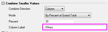
Combine Smaller Values allows smaller values to be combined into an "Other" category so as to have fewer final categories to be displayed. More details can refer to the example below.
- Combine Direction: If not "None", then choose either Row categories or Column categories to enable the feature. But combination smaller values at both row and categories is not supported currently.
- Mode: This drop-down list specifies the specific method for combining smaller values of the summarized values, which can be Count, Sum, Mean, Min or Max.
| Note: Once Mode is selected, you can also specify other supplementary options, such as Percent, Reference Row/Column Value, Top N, and Column/Row Label, beneath the Mode drop-down list, which would change according to the selected mode.
|
- By Percent of Grand Total: Row/Column categories with the percentage of the summarized value (Count/Sum/Mean/Min/Max) accounts for that of grand total exceeding a threshold percent, will be listed; while the rest will be reduced and combined into the Others category by default.You can specify the threshold percent in Percent beneath Mode drop-down list.
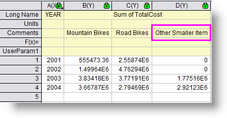
- To change the default name of the reduced category, specify the new name in Row(or Column) Label in the beneath Mode drop-down list. In the following screenshot, the default name of the reduced category has been renamed as Other Smaller Item and other categories with smaller percentages has been reduced into this category.
- By Percent of Reference Row/Column: Row/Column categories with the percentage of the summarized value in reference column/row category accounts for that of grand total exceeding a threshold percent, will be listed; while the rest will be reduced and combined into the Other(default) category. Choose one of the available value displayed to specify the reference column/row category in Reference Column/Row Value. For the customization of threshold percent and reduced column name, please refer to By Percent of Grand Total below.
- Top N of Grand Total:The summarized value of each row/column category will be ranked and the top N row/column categories will be listed. Specify the Top N and the Row(or Column) Label beneath Mode drop-down list.
- Top N of Reference Row/Column :The summarized value of each row/column category in column/row reference category will be ranked and the top N row/column categories will be listed. Specify the Top N and the Row(or Column) Label beneath Mode drop-down list.
- Reference Row/Column Value: Specify the reference row/column when either By Percent of Reference Row/Column or Top N of Reference Row/Column is selected for Mode.
- Percent: Specify the percent for qualifying the smaller values when either By Percent of Grand Total or By Percent of Reference Row/Column is selected for Mode.
- Column/Row Label: Customize the reduced category name when combining smaller values.
Options
- Total for Rows:This option would add a column for row total.
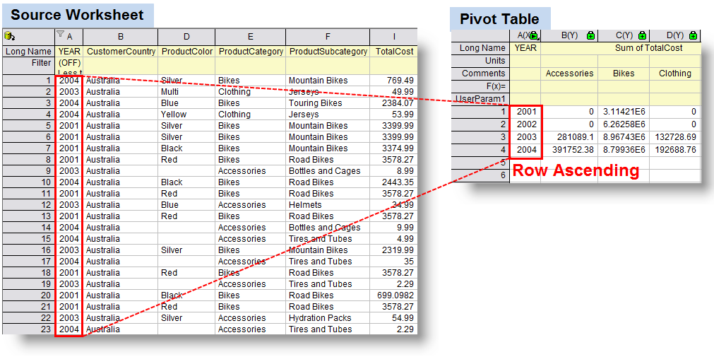
- Sort Output Rows:This option define the sort order of output rows.
- Row Label Ascending:This option will sort the rows according to the Row Labels in ascending order.
See the following example. When only using Year as the only row source, the year has been sorted in ascending way. See the following example. When more than one range is select as row sources, the pivot table would arrange the data according to the sequence of row sources.
- Row Label Ascending: This option will sort the rows according to the Row Labels in descending order, which similar to the case of Row Label Ascending but with reverse sequence of the sorting data.
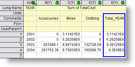
- Ascending by Row Totals: This option would sort Row Totals in ascending order. Under this circumstance, only number data is permitted to be designated in the Pivot Table Data Source. Note that this option can be selected whether the box of Totals for Rows is selected or not.
- Dscending by Row Totals: This option would sort Row Totals in dscending order. Similar to Ascending by Row Totals, only number data is permitted to be designated in the Pivot Table Data Source under this circumstance.
- None: Do not sort the rows.
- Total for Columns: Similar to Total for Rows, add a row for column total.
- Sort Output Columns:Similar to Sort Output Rows, sort according to Column Label or Column Total in ascending/descending way, if not None.
- Normalize by Column Totals
- None: Do not normalize the data.
- Fraction: Normalize the data in each column by the column total and report in fractional notation.
- Percent: Normalize the data in each column by the column total and report in percentage notation.
- Show Zero when Empty: Display 0 instead of missing values for empty cells. It is only available when Summarize by is not by Count.
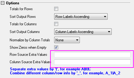
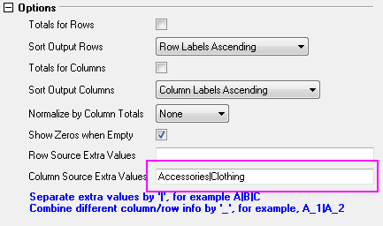
- Row Source Extra Values: This option is used less often, please refer to Column Source Extra Values below.
- Column Source Extra Values: This option provide additional categories that might be missing in the source data column. This is useful when you want to ensure all needed categories will be present in the result table. Categories missing in the input data may show as 0 (when summarized by count and sum) or missing values "--" (when summarized by min or max).
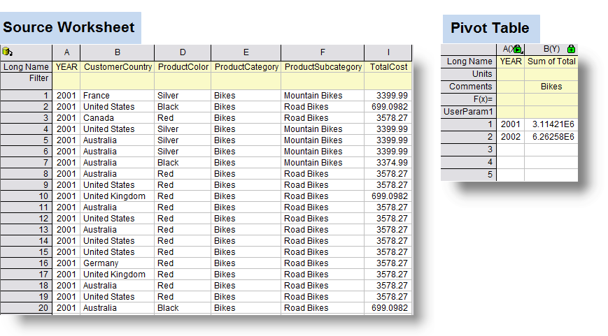
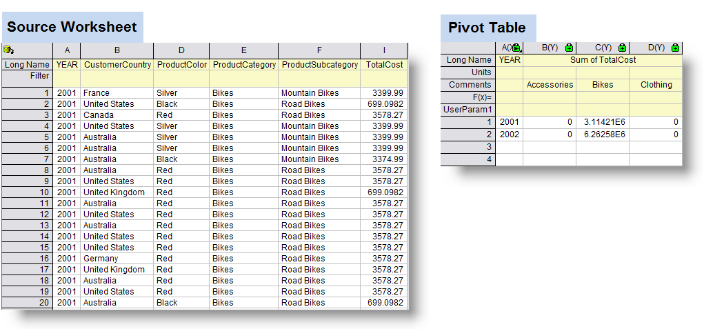
Suppose you have the following dataset(See source worksheet in the screenshot below). It is sales summary of several products(Bike, Accessories,and Clothing) in different countries from year 2001 to year 2004. You want to create a summary presenting the total cost of different products on each year. You can specify YEAR as column category and Categories as row category. However, the sales record of Accessories and Clothing in 2001 and 2002 are missing. The following two situations display the different result of whether or not using Column Source Extra Values.
- Without Column Extra Values
- If using the worksheet query to display the data with Condition as: YEAR <= 2002, then create a pivot table of sum of total cost without specifying Column Extra Value based on the new extracted query data. The pivot table would exclude the category Accessories and Clothing, only displaying the category Bikes, which has extant data record of YEAR 2001 and 2002 in the source worksheet.
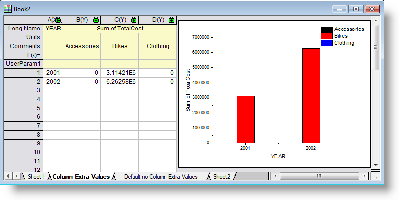
- On the contrary, if creating a similar pivot table but specifying the Column Extra Value, the pivot table would display all three categories, despite of missing records. These two missing categories would be shown with zero sum.
| Note:
Column Extra Value feature is extremely important when you are using the pivot table to plot a graph. In this situation, you might want all categories presented even if the records of some categories in source worksheet is not complete. Setting Column Extra Value would automatically treat the missing data as zero but still regard the related categories as data groups in the graph.
|
- Put Column Info. to: The names of column categories will be put into the pivot table Comment column label row by default, But categories name can be put into the any column label rows you specified in this drop-down list.
- Long Name: Output column categories name into Long Name column label row.
- Comments: Output column categories name into Comment column label row.
- Append to Column's Long Name: Append the Long Name of column category in source worksheet to the Long Name column label row in pivot table.
- User Defined Parameters: Output other information (Short Name or Long Name of column categories in source worksheet) of the column categories into User Defined Parameters column label row in pivot table.
- From Column: Specify the source value of User Defined Parameters,only available when User Defined Parameters selected from Put Column Info. to.
- Short Name: Choose Short Name of column categories in source worksheet as input information for User Defined Parameters.
- Long Name: Choose Long Name of column categories in source worksheet as input information for User Defined Parameters.
Output Result Table to
Specify where to output the result pivot table. Click the triangle button to specify output method.
[<input>]<input>: Input the pivot table into the current worksheet.
<new>: Put pivot table into a new sheet of the current workbook.
[<new>]<new>: Put pivot table into a new workbook.
|