15.3.6.1 Parameter InitializationFitPara-INI
The Levenberg-Marquardt iterative algorithm requires initial values to start the fitting procedure. Good parameter initialization results in fast and reliable model/data convergence. When defining a fitting function in the Function Organizer, you can assign the initial values in the Parameter Settings box, or enter an Origin C routine in the Parameter Initialization box with which the initial values can be estimated.
The NLFit in Origin provides automatic parameter initialization code for all built-in functions. For user-defined functions, you must add your own parameter initialization code. If no parameter initialization code is provided, all parameter values will be missing values when NLFit starts. In this case, you must enter "guesstimated" parameter values to start the iterative fitting process.
Note that initial parameter values estimated by parameter initial routines will be used even if different initial values are specified in Parameter Settings.
Set initial values in Parameter Settings dialog
Click the  button beside Parameter Settings box to bring up the Parameter Settings dialog. Then you can enter proper initial values for the parameters in the Value column of Parameters tab: button beside Parameter Settings box to bring up the Parameter Settings dialog. Then you can enter proper initial values for the parameters in the Value column of Parameters tab:
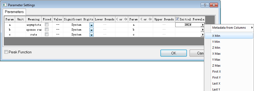
To initialize parameters by initial formula (column statistics values, label rows, .etc), you can check the Initial Formula column check box and select the desired initial formula or metadata from the fly-out menu.
Estimate parameter initial values by Origin C code
The text box in Parameter Initialization contains the parameter initialization code. For built-in functions, these routines can effectively estimate parameter values prior to fitting by generating dataset-specific parameter estimates. When defining a new Origin C fitting function, you can edit the initial codes in the code builder by clicking the button.
Although there many methods to estimate the parameter initial values, in general we will transform the function and deduce the value based on the raw data. For example, we can define a fitting model, named MyFunc, as:

(This is the same function like the built-in Allometric1 function in Origin)
And then transform the equation by:
=\ln (ax^b)\,\!") =\ln (a)+b\ln (x)\,\!")
After the transformation, we will have a linear relationship between ln(y) and ln(x), and the intercept and slope is ln(a) and b respectively. Then we just need to do a simple linear fitting to get the estimated parameter values. The initial code can be:
#include <origin.h>

void _nlsfParamMyFunc(
// Fit Parameter(s):
double& a, double& b,
// Independent Dataset(s):
vector& x_data,
// Dependent Dataset(s):
vector& y_data,
// Curve(s):
Curve x_y_curve,
// Auxilary error code:
int& nErr)

{                                                  // Beginning of editable part
	sort( x_y_curve );                         // Sort the curve
	Dataset dx;
	x_y_curve.AttachX(dx);                     // Attach an Dataset object to the X data
	dx = ln(dx);                               // Set x = ln(x)
	x_y_curve = ln( x_y_curve );               // Set y = ln(y)
	vector coeff(2);
	fitpoly(x_data, y_data, 1, coeff);         // One order (simple linear) polynomial fit
	a = exp( coeff[0] );                       // Estimate parameter a
	b = coeff[1];                              // Estimate parameter b
                                                   // End of editable part
}
In the Code Builder, you just need to edit the function body. The parameters, independent variables and dependent variables are declared in the function definition. In addition, a few Origin objects are also declared: A dataset object is declared for each of the independent and dependent variables and a curve object is declared for each xy data pair:
vector& x_data;
vector& y_data;
Curve x_y_curve;
The vectors represent cached input x and y values, which should never be changed. And the curve object is a copy of the dataset curve that is comprised of an x dataset and a y dataset for which you are trying to find a best fit.
Below these declaration statements, there is an editable section; the white area; which is reserved for the initialization code. Note that the function definition follows the C syntax.
| Note: The function is of type void, which means that our function returns no values. The parameter variables are stored in the function code.
|
Initialization is accomplished by calling built-in functions that take a vector or a curve object as an argument. Once the initialization function is defined, you should verify that the syntax is correct. To do this, click the Compile button at the top of the workspace. This compiles the function code using the Origin C compiler. Any errors generated in the compile process are reported in the Code Builder Output window at the bottom of the workspace.
Once the initialization code has been defined and compiled, you can return to the Function Organizer interface by clicking on the Return to Dialog button at the top of the workspace.
Note: If you wish to debug your code, you can open the initialization code in Code Builder from Code Tab of NLFit dialog and set break points. Then click Initialize Parameters button  to call and debug initialization code. For further information on debugging, select Help:Programming:Code Builder… from the Origin menu and search on debug. to call and debug initialization code. For further information on debugging, select Help:Programming:Code Builder… from the Origin menu and search on debug.
|
Frequently Used Origin C Function for Parameter Initialization
| Function
|
Description
|
|
area
|
Get the area under a curve.
|
|
Curve_MinMax
|
Get X and Y range of the Curve.
|
|
Curve_x
|
Get X value of Curve at specified index.
|
|
Curve_xfromY
|
Get interpolated/extrapolated X value of Curve at specified Y value.
|
|
Curve_y
|
Get Y value of Curve at specified index.
|
|
Curve_yfromX
|
For given Curve returns interpolated/extrapolated value of Y at specified value of X.
|
|
fitpoly
|
Fit a polynomial equation to a curve (or XY vector) and return the coefficients and statistical results.
|
|
fit_polyline
|
Fit the curve to a polyline, where n is the number of sections, and get the average value of X-coordinates of each section.
|
|
fitpoly_range
|
Fit a polynomial equation to a range of a curve.
|
|
find_roots
|
Find the points with specified height.
|
|
fwhm
|
Get the peak width of a curve at half the maximum Y value.
|
|
get_exponent
|
This functions is used to estimate y0, R0 and A in y = y0 + A*exp(R0*x).
|
|
get_interpolated_xz_yz_curves_from_3D_data
|
Interperate 3D data and returns smoothed xz, yz curves.
|
|
ocmath_xatasymt
|
Get the value of X at a vertical asymptote.
|
|
ocmath_yatasymt
|
Get the value of Y at a horizontal asymptote.
|
|
peak_pos
|
This function is used to estimate the peak's XY coordinate, peak's width, area.etc.
|
|
sort
|
Use a Curve object to sort a Y data set according to an X data set.
|
|
Vectorbase::GetMinMax
|
Get min and max values and their indices from the vector
|
|
xatasymt
|
Get the value of X at a vertical asymptote.
|
|
xaty50
|
Get the interpolated value of X at the average of minimum and maximum of Y values of a curve.
|
|
xatymax
|
Get the value of X at the maximum Y value of a curve.
|
|
xatymin
|
Get the value of X at the minimum Y value of a curve.
|
|
yatasymt
|
Get the value of Y at a horizontal asymptote.
|
|
yatxmax
|
Get the value of Y at the maximum X value of a curve.
|
|
yatxmin
|
Get the value of Y at the minimum X value of a curve.
|
More Parameter Initialization Examples
Exponent function
Sample Function
- EXPDEC2
Equation

Initialization Code
int sign;
t1 = get_exponent(x_data, y_data, &y0, &A1, &sign);
t1 = t2 = -1 / t1;
A1 = A2 = sign * exp(A1) / 2;
Description
Because most of the exponential curves are similar, we can use a simple exponential function to approach complex equations. This EXPDEC2 function can be treated as the combination of two basic exponential function, whose parameters comes from get_exponent.
Peak function
Sample Function
- LORENTZ
Equation
^2+w^2}")
Initialization Code
xc = peak_pos(x_y_curve, &w, &y0, NULL, &A);
A *= 1.57*w;
Description
In this initialization code, we firstly evaluate the peak width  , baseline value , baseline value  , peak center , peak center  and peak height, which is originally assign to the variable and peak height, which is originally assign to the variable  , by the peak_pos function. And then compute the peak area, A, by the following deduction: , by the peak_pos function. And then compute the peak area, A, by the following deduction:
Let  is the value where is the value where  , then we have: , then we have:

and

Where H is the peak height.
Sigmoidal Function
Sample Function
- DRESP
Equation
p}}")
Initialization Code
sort(x_y_curve);
A1 = min( y_data );
A2 = max( y_data );
LOGx0 = xaty50( x_y_curve );
double xmin, xmax;
x_data.GetMinMax(xmin, xmax);
double range = xmax - xmin;
if ( yatxmax(x_y_curve) - yatxmin(x_y_curve) > 0)
	p = 5.0 / range;
else
	p = -5.0 / range;
Description
Knowing the parameter meanings is very helpful and important for parameter initialization. In the does-response reaction, A1 and A2 means the bottom and top asymptote respectively, so we can initialize them by the minimum and maximum Y values. The parameter LOGx0 in the reaction is a typical value that 50% reaction happens, that's why we use the xaty50 function here. Regards to the slope, p, it doesn't matter how you compute this value, however, the sign of the slope is important.
Surface Function
Sample Function
- Gauss2D
Equation
^2-\frac{1}{2}(\frac{y-y_c}{w_2})^2}")
Initialization Code
Curve x_curve, y_curve;
bool bRes = get_interpolated_xz_yz_curves_from_3D_data(x_curve, y_curve, x_data, y_data, z_data, true);
if(!bRes) return;
xc = peak_pos(x_curve, &w1, &z0, NULL, &A);
yc = peak_pos(y_curve, &w2);
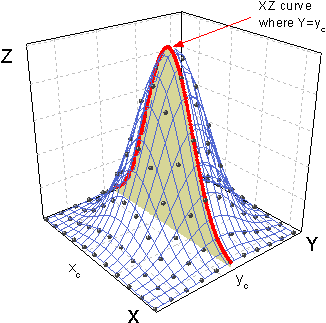
Description
One idea for evaluating surface function initial values is solving the problem in a plane. Take this Gauss2D function as example, it's quite obviously that the maximum Z value is on the point (xc, yc), so we can use the get_interpolated_xz_yz_curves_from_3D_data function to get the characteristic curve on XZ and YZ plane. And then use the peak_pos function to evaluate the other peak attributes, like peak width, peak height, etc.
|