17.2.7 2D Kernel Density

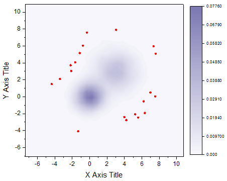
The 2D Kernel Density plot is a smoothed color density representation of the scatterplot, based on kernel density estimation, a nonparametric technique for probability density functions. The goal of density estimation is to take a finite sample of data and to infer the underyling probability density function everywhere, including where no data point are presented. In kernel density estimation, the contribution of each data point is smoothed out from a single point into a region of vicinity. These smoothed density plot shows an average trend for the scatter plot.

1 Creating 2D Kernel Density Plot
2 The Dialog of plot_kde2
3 Algorithm

Creating 2D Kernel Density Plot

To create a 2D Kernel Density plot:

Highlight one Y column.
Open 2D Kernel Density plot dialog by clicking Plot > Contour: 2D Kernel Density.
In the plot_kde2 dialog box, specify the Method , Number of Grid Points in X/Y and the Number of Points to Display, and Plot Type.
Click OK to create a 2D Kernel Density plot.

The Dialog of plot_kde2

Input Data	Specify the input data.
Settings	Bandwidth Method Specify the bandwidth calculation method of the 2D Kernel Density plot. Bivariate Kernel Density Estimator Rules of Thumb Density Method Specify a method to calculate the kernel density for defined XY grids. Exact Estimation Choose the option to calculate density values according to the Ks2density equation. For a large dataset, computation of the exact computation may require extensive calculation, Binned Approximate Estimation Choose the option to calculate approximation of density values. This option is recommended for a large sample. Number of Points to Display Specify the first N lowest density points to be superimposed on the density image. Interpolate Density Points Specify the calculation method to decide which points to superimposed on the density image (see details in below Algorithm section). Usually if the number of source data is large (ie. >50000), we strongly recommend to select this option to improve the speed. Number of Grid Points in X/Y Specify the number of equally spaced grid points for the density estimation. Number of Points to Display Specify the first N lowest density points to be superimposed on the density image when the checkbox of All is unchecked. Otherwise, it will display all points when the All checkbox is selected by default. Grid Range As an interim step, a matrix of gridded values is generated from the X/Y data and the kernel density plot is created from the matrix values. By default, the Grid Range registers the minimum and maximum X and Y values in that matrix. Clear the Auto box to enter a value manually. X Minimum X Maximum Y Minimum Y Maximum Plot Type Specify the plot type. Contour Use the density matrix to plot contour Image Use the density matrix to make an image plot
Density Estimation data	This determines where the calculated data for the graph is stored.
Displaying Data	This determines where the data of the displayed scatter plot is stored. Only available when Number of Points to Display is not 0.

Algorithm

Kernel density estimation is a nonparametric technique to estimate density of scatter points. The goal of density estimation is to estimate underlying probability density function everywhere, including where no data are observed, from the existing scatter points. A kernel function is created with the datum at its center – this ensures that the kernel is symmetric about the datum. Kernel density estimation smooths the contribution of data points to give overall picture of the density of data points.

Density Calculation Method

Specify a method to calculate the kernel density for defined xy grids.

Exact Estimation

Density values are calculated based on the equation below

$f(x,y,\text{vX},\text{vY},w_x,w_y) = \frac{1}{n} \sum_{i=1}^{n} \frac{1}{ 2\pi w_x w_y } \exp \left(-\frac{(x-\text{vX}_i)^2}{2w_x ^2} - \frac{(y-\text{vY}_i)^2}{2w_y^2} \right)$

where n is the number of elements in vector vX or vY, $\text{vX}_i$ is ith element in vector vX and $\text{vY}_i$ is ith element in vector vY. $w_x$ and $w_y$ is the optimal bandwidths values.

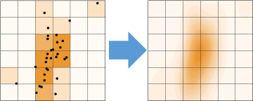
Binned Approximate Estimation

Speed up the density calculation by an approximation to the exact estimation of 2D kernel density.

First 2D binning is performed on the (x, y) points to obtain a matrix with the bin counts. Then 2D Fast Fourier Transform is utilized to perform discrete convolutions for calculating density values of each grid.

4th root of density values is calculated to map the density scale to the color scale

Bandwidth Methods

Bivariate Kernel Density Estimator

Calculate bandwidth based on linear diffusion process.

Rule of Thumb

The estimation of wx and wy simply can be calculated by:

$w_x = \frac{\sigma_x}{2n^{1/6}}$

$w_y = \frac{\sigma_y}{2n^{1/6}}$

where n is the size of vector vX or vY, $\sigma_x$ is the sample standard variation for dataset vX, and $\sigma_y$ for dataset vY accordingly.

Interpolate Density Points

Specify the calculation method to decide which points to superimpose on the density image.

If the option is selected, kernel density of points are calculated by the interpolation on the density matrix for defined XY grids. If number of source data is very large, selecting the option can greatly improve the speed.

If the option is not selected, the density values will be calculated by the Exact Estimation method.

Skip Navigation Links

All Books