8.11.2 Creating Contour GraphsCreate-Contour-Graph
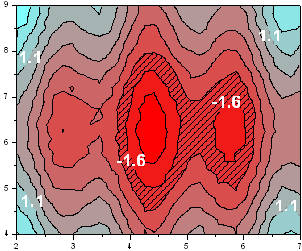
Contour graphs are surface graphs plotted in 2D space. Viewing a contour graph is the same as viewing a 3D surface graph from a vantage point perpendicular to the XZ plane. In contour graphs, ranges of Z values are distinguished by different colors or levels of gray scale, labeled contour lines, or both.
Contour Graph Types
Origin provides seven contour graph types:
| Graph Type
|
XYZ Columns in Worksheet
|
Matrix Window
|
Virtual Matrix in Worksheet
|
- Countour-Color Fill
- Contour - B/W Lines+Labels
- Gray Scale Map
- Heatmap
|
Yes (except Heatmap)
|
Yes
|
Yes
|
- Polar Contour thea(x)r(y)
|
Yes
|
Yes
|
No
|
- Polar Contour r(x)thea(y)
- Ternary Contour
|
Yes
|
No
|
No
|
The (Plot Details) Color Map/Contours and Label tabs provide controls for editing your contour graphs.
Note that a contour plot in Origin can be created from matrix data, worksheet data, or virtual matrix data. Creating a contour plot from a matrix is faster than creating a contour plot directly from a worksheet, so the matrix method is suitable for large data. On the other hand, creating a contour plot directly from XYZ worksheet data uses a triangulation method to generate the contour lines, and there is no need to generate a matrix.
| Note: A contour triangulation algorithm that plots raw X and Y data was implemented for Origin 2016. Previous versions performed some normalization of X and Y data before plotting. Thus, contour and 3D surface plots of XYZ worksheet data, created in version 2016 and higher, may differ from plots of the same data created in earlier versions. This change will be most noticeable if there are large scale range differences between X and Y values. See FAQ-822 for more information.
|
Other advantages to creating contour graphs from XYZ worksheets:
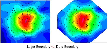
- Supports Layer Boundary, Data Boundary and Custom Boundary.
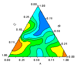
- Supports Ternary Contour Plots
Contour graphs created from XYZ data or a virtual matrix support nonlinear X/Y axes while those from a matrix window only support linear axes.
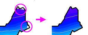
 | Prior to Origin 2018, the application of a custom boundary sometimes generated an imperfect fill at boundary margins. This has been improved in 2018. The user can restore the previous contour-fill behavior using system variable @TCSM.
|
How to Create and Customize Contour Graphs
To create a Contour graph from matrix data, click the appropriate graph button or select the appropriate option in the Plot menu. To create a Contour graph from XYZ data, select a Z column or select no columns and pick one of the two above methods. To create a graph from virtual matrix data, you must select all the source data in your worksheet and use one of the two above methods which will open a dialog which will create the internal virtual matrix and graph. For more details about creating graphs from virtual matrices, please refer to Creating 3D and Contour Graphs from Virtual Matrix. We also explain each Contour graph type in detail in Contour Graphs.
Customizations of Contour graphs are handled by the Axis dialog and the Plot Details dialog. You can get more details about the Axis dialog from Graph Axes. To get more details about the Plot Details dialog, please refer to Customizing Your Graph.
The Highlight Features for Contour Graphs
There are some special features of contour graphs.
Extract Data Points from Contour Plot
XYZ Contour
Once you created a contour plot from XYZ data, you can right click on the contour plot and select Extract Data Points to open Extract Data Points: xyzgrid dialog. Then you can specify the grid sizes and ranges along X and Y directions/ specify X and Y from Columns/ pick up points in the contour, and then output the interpolated data at specified grid points in either XYZ or matrix form to a new book.
The values for the specified grid points are computed by triangulation and line interpolation as described in algorithm section.
Note that contour values outside input data range will be set as missing values.
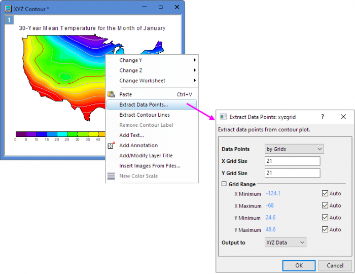
Dialog Controls of the Extract Data Points: xyzgrid Dialog
| Data Point
|
Specify the methods to extract data points.
- by Grids
- by Columns
- Pick from Graph
|
| X Grid Size
|
When choose extract data points by Grids, specify the number of grid points along X direction.
|
| Y Grid Size
|
When choose extract data points by Grids, specify the number of grid points along Y direction.
|
| Grid Range
|
When choose extract data points by Grids, specify the boundary of the input data range. By default, all data points are included. In order to exclude bad or unwanted data points, you can restrict the input data range by editing the minimum and maximum XY coordinates (Note: Contour values outside input data range will be treated as missing values.).
- X Minimum
- the minimum X value of the output XYZ/matrix data.
- X Maximum
- the maximum X value of the output XYZ/matrix data.
- Y Minimum
- the minimum Y value of the output XYZ/matrix data.
- Y Maximum
- the maximum Y value of the output XYZ/matrix data.
|
| Output to
|
Specify the output data form:
- XYZ Data
- Output interpolated contour values in XYZ data form.
- Matrix
- Output interpolated contour values in matrix form.
|
| Input
|
When choose extract data points by Columns, specify the columns of X and Y range for extracting the corresponding Z value.
|
| Output to
|
Specify the output data to:
- Same Sheet of XY
- New Sheet
|
| Pick
|
When choose extract data points Pick from Graph, click this Pick button, and then double-click on the graph to select the points you want to extract. Then click Done button, it will extract the XYZ of the points in a new sheet.
|
Virtual Matrix or Matrix Contour
Once you created a contour plot from virtual matrix or matrix, you can right click on the contour plot and select Extract Data Points to open Extract Data Points: mgrid dialog. Then you can specify the grid sizes and ranges along X and Y directions/ specify X and Y from Columns/ pick up points in the contour, how to treat the missing values, and output the interpolated data at specified grid points in matrix form to a new book.
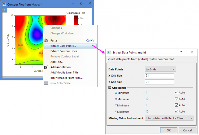
Dialog Controls of the Extract Data Points: mgrid Dialog
| Data Point
|
Specify the methods to extract data points.
- by Grids
- by Columns
- Pick from Graph
|
| X Grid Size
|
When choose extract data points by Grids, specify the number of grid points along X direction.
|
| Y Grid Size
|
When choose extract data points by Grids, specify the number of grid points along Y direction.
|
| Grid Range
|
When choose extract data points by Grids, specify the boundary of the input data range. By default, all data points are included. In order to exclude bad or unwanted data points, you can restrict the input data range by editing the minimum and maximum XY coordinates (Note: Contour values outside input data range will be treated as missing values.).
- X Minimum
- the minimum X value of the output matrix data.
- X Maximum
- the maximum X value of the output matrix data.
- Y Minimum
- the minimum Y value of the output matrix data.
- Y Maximum
- the maximum Y value of the output matrix data.
|
| Missing Value Pretreatment
|
Specify the method to preprocess missing values when generate grid data with interpolation.
- Skip
- Remove all missing values first and then run interpolation.
- Interpolated with Renka Cline
- Renka Cline: For an arbitrary point P, compute the interpolated value using the data values and gradient estimates at each of the three vertices of the triangle which contains P.
|
| Input
|
When choose extract data points by Columns, specify the columns of X and Y range for extracting the corresponding Z value.
|
| Output to
|
Specify the output data to:
- Same Sheet of XY
- New Sheet
|
| Pick
|
When choose extract data points Pick from Graph, click this Pick button, and then double-click on the graph to select the points you want to extract. Then click Done button, it will extract the XYZ of the points in a new sheet.
|
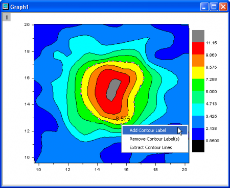
Adding or Removing Contour Labels
- If adding to only one or two contours, you can do it this way:
- Press CTRL + SHIFT and click precisely on the contour line that you want to label. Right-click and choose Add Contour Label.
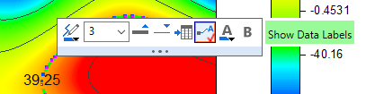
- Click twice (do not double-click) on a contour line and popup a Mini Toolbar for single-level customization.
- Adjust label position by dragging.
To remove (hide) contour labels:
- Use the controls on the Color Map/Contours tab. You can also click the Mini Toolbar's Show Contour Labels button
 to toggle contour label display. to toggle contour label display.
- Alternately: To remove all labels from a contour level, press CTRL + click precisely on a level, then right-click and choose Remove Contour Label(s). To remove labels from a single contour line (i.e. within a contour level), press CTRL + SHIFT to select the line, then right-click and choose Remove Contour Label(s).
Extracting Contour Lines
Extract Contour Lines outputs the Z value, the XY coordinates and the area enclosed by the contour, to a new worksheet. The area calculation is done by the Polygon Area (polyarea) X-Function. Polygon Area returns the area enclosed by a given contour (Z value). There is no subtraction of the area within included contours.
To extract contour lines:
- Click once to select all contour lines;
- Click a second time to select all contour lines at a given Z value;
- Click a third time to select a single contour line;
... then, right-click on your selection and choose Extract Contour Lines. Contour data, including contour area, are output to a new workbook.
Algorithm for Creating a Contour from a Worksheet
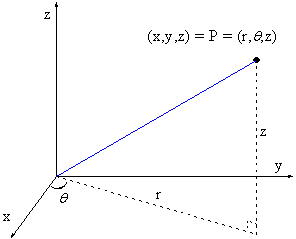
Contour plots can be created directly (without gridding) from (x, y, z) coordinates (Cartesian coordinates) or (r,  , z) coordinates (cylindrical coordinates). If your data are in (r, , z) coordinates, Origin first converts the data to XYZ space before making the contour plot. Conversions between (x, y, z) and (r, , z) coordinates are expressed as: , z) coordinates (cylindrical coordinates). If your data are in (r, , z) coordinates, Origin first converts the data to XYZ space before making the contour plot. Conversions between (x, y, z) and (r, , z) coordinates are expressed as:

")

and...


In Cartesian space, creating a contour plot is a four step process:
- Drawing of contour lines.
- Connecting and smoothing.
Triangulation
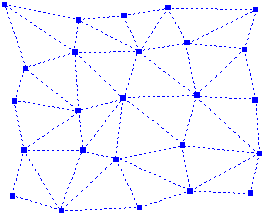
All data points are connected to create Delaunay triangles in the XY plane. The triangles are constructed so as to make them as equiangular as possible. In addition, no two triangles should intersect. Note that any side is shared by two adjacent triangles, unless it is located at the edge of the mesh.
Linear interpolation
To find the intersection points of the contour lines and the triangle sides:
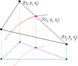
Given a contour level zc, Origin traverses all the triangles to see whether or not the contour line for this level intersects with the triangle sides. If a triangle side has intersection with the contour line, it will be marked as a characteristic side. The coordinates of the intersection point, which will be referred to as a characteristic point in this document, will be computed with linear interpolation.
For a triangle side that connects two triangle vertices: I(xi, yi, zi) and J(xj, yj, zj), we will examine whether the following is true:
 *\left( z_j-z_c\right) <0")


If it is true, we will say that this side is a characteristic side. Furthermore, if the product on the left of the inequality is zero, it will mean that the contour line passes through at least one of the vertices. In this case, zi and zj will be adjusted by subtracting a small value,  , so as to make sure that the characteristic point will not be a vertex. The adjustment is as follows: , so as to make sure that the characteristic point will not be a vertex. The adjustment is as follows:
where  . .
If this side is a characteristic side, the coordinates of the characteristic point on it can be computed by linear interpolation in the following way:
")
")
Origin keeps records of all the characteristic sides and the coordinates of the characteristic points for future use.
Note that if a triangle intercepts the contour line, it will have exactly two characteristic sides.
Drawing of contour lines
To draw a contour line, we have to trace all the characteristic points on it.
If there is a characteristic point on the boundary of the triangular mesh, the tracing will start from that point. Otherwise, the tracing will begin with a random characteristic point.
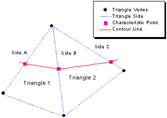
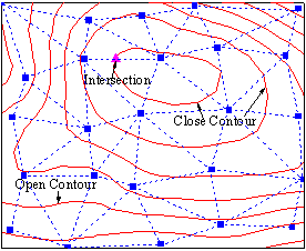
Recall that a triangle that intercepts the contour line must have exactly two characteristic sides, and that a side which is not on the edge of the mesh must be shared by two triangles. Therefore, the tracing can go from one characteristic side (Side A in the following figure) to the other characteristic side of the same triangle (Side B in the following figure). If the latter is not on the edge of the triangular mesh, we will certainly find another triangle (Triangle 2 in the following figure) which shares this side with the current triangle (Triangle 1 in the following figure). Then we can find the characteristic point on the other characteristic side (Side C in the following figure) of this new triangle. In this way, the tracing continues until the edge of the mesh or a characteristic point which has already been traced is reached. (In the former case, the contour line is open; while in the latter case, it is closed.) Then the number of characteristic points that have been traced is compared with the total number of characteristic points for this level. If they are not equal, it will mean that there are still some characteristic points which have not been traced. The tracing will go on until all characteristic points have been traced.
Connecting and smoothing
After the tracing, the characteristic points are connected with straignt lines. Then smoothing is available for Contour from a Worksheet when the Smoothing checkbox in Plot Details dialog Contouring Info tab is ticked. You can read the imformation about smoothing parameters and the TPS algorithm, which is used for
Contour from a Worksheet.
Algorithm for Creating a Contour from a Matrix
Creating a contour from matrix (or virtual matrix) has a similar but simpler algorithm, there are only three steps:
- Drawing of contour lines.
In which the linear interpolation, drawing of contour lines are just the same as the algorithm to create contour from workbook as explained above.
As for the line connection, when creating contour from matrix, the characteristic points are connected with straight lines. And no smoothing is performed afterwards.
Reference:
- Robert J. Renka. Interpolation of Data on the Surface of a Sphere. ACM Transactions on Mathematical Software, Vol. 10, No. 4, December 1984, Pages 417-436.
- Fen Yuan, Automatic Drawing of Equal Quantity Curve. Computer Aided Engineering, No. 3 Sept. 1998.
|