6.5.3 Scatter Plot of Decay and Recovery Curves

Customize-Grouped-Scatter

Adding, Grouping and Reordering Plots with Layer Contents Group and Ungroup Plots in Object Manager Customize Legend Symbol How to customize legend symbols and user-defined legend entries

Summary

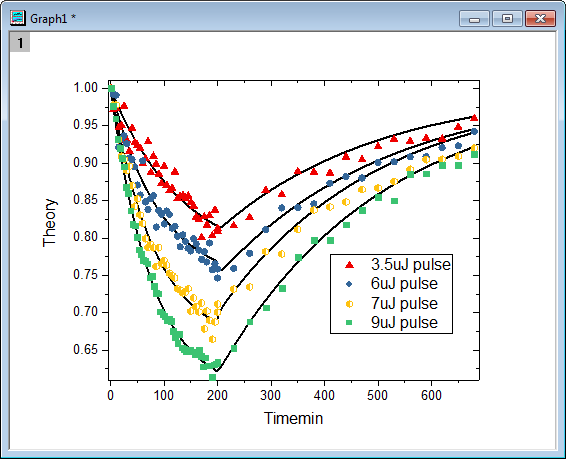
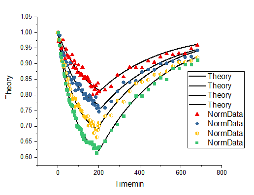
The scatter plot below depicts 3 decay and recovery curves obtained after taking two-photon fluorescence measurements of reversible photodegradation in a dye-doped polymer. To learn more about the graph, please read the case study.

Minimum Origin Version Required: Origin 2016 SR0

What you will learn

• How to use the Plot Setup dialog to arrange plots in a layer
• How to customize the symbols in your graph

Steps

1. Download the zip file from here and extract the text files .
2. Open Origin and click the Import Multiple ASCII button on the Standard toolbar to open the ASCII dialog and then import the text files.
   
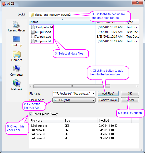
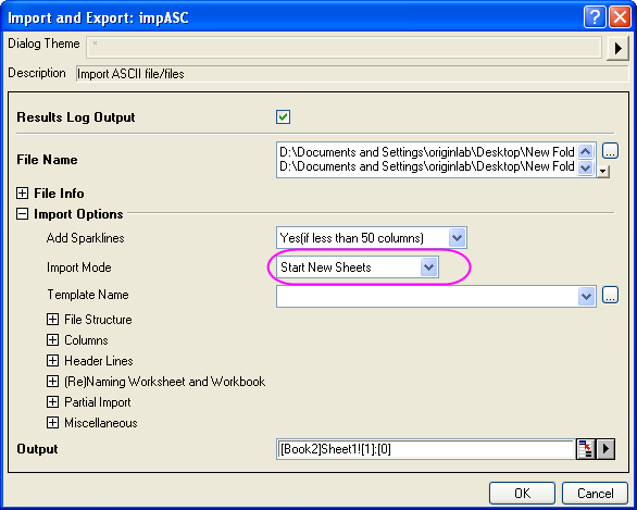
3. In the impASC dialog, set Import Mode as Start New Sheets. Click OK to finish importing.
   
4. We will use the Plot Setup dialog to create a graph with 8 plots. Active the workbook, and make sure that no datasets are now selected. Click the button on the 2D Graphs toolbar to open the Pot Setup dialog.
   Show all of the three panels of Plot Setup dialog (if not all of them are shown) by clicking the and buttons.
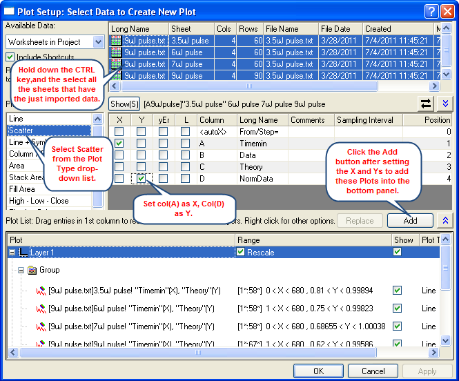
   First, we will add 4 line plots into a graph by using the Plot Details dialog. Highlight all dataset in the top panel, and then select column Timemin as X, column Theory as Ys in the middle panel. Then add them into the bottom panel.
   Then we will add 4 scatter plots in to the same graph. Select Scatter from the Plot Type drop-down list, make sure all dataset in the top panel has been selected, and then select column Timemin as X, column NormData as Ys in the middle panel. Then add them into the bottom panel.
   

   In order to show all three panels in Plot Setup dialog, please expand Plot Type panel by clicking and expand Available Data panel by clicking again. Please refer to Plotting using Plot Setup for more information.

   
   In bottom panel, if there is a Group branch under Layer1, right-click on it to select Ungroup from the short-cut menu to ungroup these plots.
   
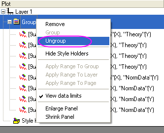
   Click OK to generate the graph which look like the following image shows.
   

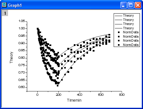
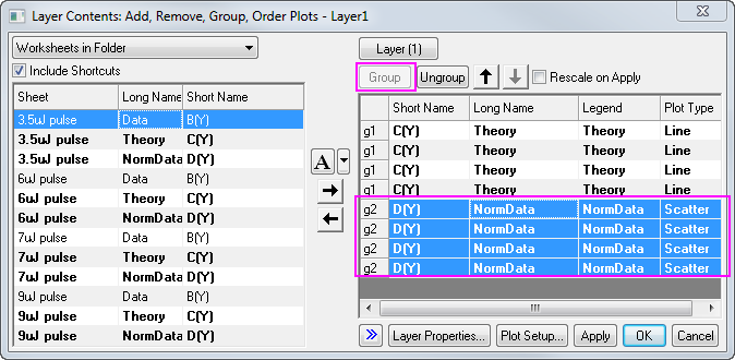
5. Double-click the layer icon at the top-left corner of graph window to open the Layer Contents dialog. Then group the Theory plots and NormData Plots as Group 1 and Group 2 using the Group button after highlight the 4 Theory/Norma Data plots separately by using mouse and the Shift key,
   
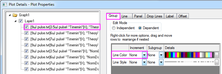
6. Then we will customize the 8 plots in the Plot Details dialog. Select Format: Plot to open the Plot Details dialog. In the left panel of the dialog, you could see there are 8 plots: the first 4 plots are line plots, the other 4 are scatter plots.
7. We will first customize the 4 line plots. Open Plot Details by double clicking the plot. On the left panel, 4 line plots are put ahead of the 4 scatter plots. You can select the first line plot by selecting the first plot under Layer 1 in this panel then go to Line tab. Select B-Spline from the Connect drop down list and set the Width to 3. Then click the Apply button. In the Group tab, select None for the increment cell in Line Color row. Click OK to apply these settings.
   
8. Then customize the 4 scatter plots. Go to Plot Detail and then select the fifth plot in the left panel, which should be the first scatter plot. Go to Symbol tab, change the Size to 8 and Edge Thickness to 0.
   In the Group tab, we will mainly customize the symbols in the list box that in the middle of the tab. In the Symbol Type row, select By one in the Increment column. Click the button to open the Increment Editor dialog, in the dialog select UpTriangle, Circle,Hexagon and Square for the first 4 rows.
   In the Symbol Edge Color row, select By one in the Increment column. In the Details column, click the color list to select the list Q11: Candy from the color list drop-down list.
   In the Symbol Interior row, select By one in the Increment column. Click the button to open the Increment Editor dialog, in the dialog select Solid, Solid,Half Left and Solid for the first 4 rows. Click OK button to close the Plot Details dialog, then the graph will look like.
   
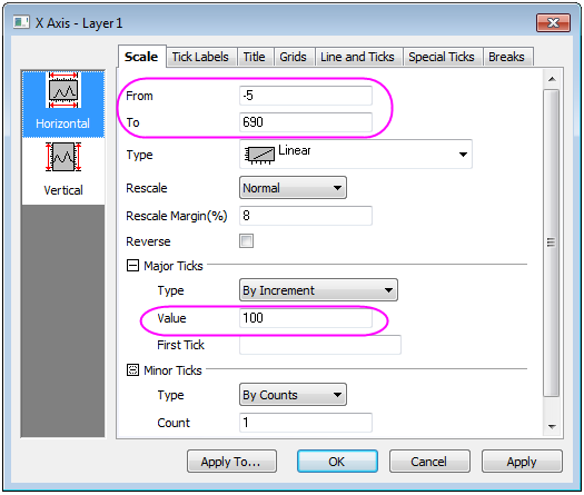
9. Then customize the Axes of the graph. Double click on the X axis to enter Axis Dialog.
   First, we customize the axes scale. Go to Horizontal icon in Scale tab, change From to -5, To to 690; set Major Ticks Type as By Increment and Value as 100, respectively. Repeat these steps to customize the Y axis range ( the Vertical icon) as From to 0.61 and To to 1.01, and Value as 0.05.
   
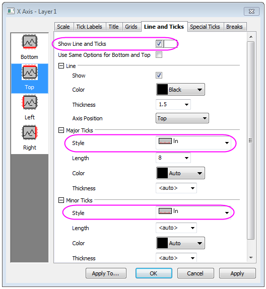
   To customize the Axis Ticks, select Top icon in Line and Ticks tab, enable the Show check box, then go to Top icon in Line and Ticks tab, select In from both Major Ticks and Minor Ticks drop-down lists. Repeat the same steps for Right Axis under Right icon.
   
10. Then you will will customize the titles and the legend. Change the titles follows the images shows. Right click on the legend and select Legend:Update Legend from the context menu to open legendupdate dialog. In this dialog, do the following:
    
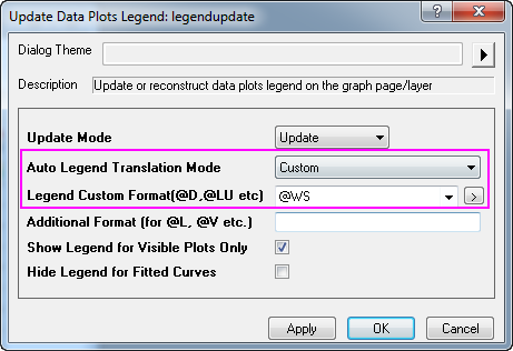
    Click Ok to close this dialog. Then the legend will update. Double-click on it to turn to the in-place edit mode, remove the first four rows.
    The final graph will look like