16.5 2D Interpolate/Extrapolate

1 Overview
- 1.1 Interpolate From XY
  - 1.1.1 To Interpolate Z from XY
  - 1.1.2 Dialog Options for Interpolate Z from XY
- 1.2 2D Interpolation on Matrix

Overview

2D Interpolation/Extrapolation allows you to interpolate/extrapolate either on a group of existing XYZ data for a given XY dataset or a specified matrix object.

Interpolate From XY

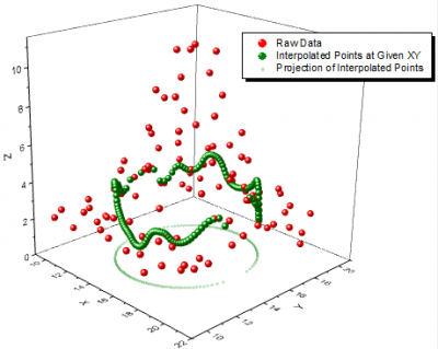
Interpolate Z From XY tool allows you to specify a set of XY values for interpolation/extrapolation so that it offers additional freedom in 2D interpolation/extrapolation for non-uniformly spaced XY dataset. Origin supports 8 interpolation methods for interpolating Z from XY: Nearest, Random Kriging, Random Renka Cline, Random Shepard, Random TPS, Spline, Triangle, Weight Average.

To Interpolate Z from XY

Activate the workbook that contains your input data.
Select Analysis: Mathematics: Interpolate Z from XY... from the menu. This opens the interp2 dialog box.
Choose your input options and click OK. The X-Function interp2 is called to complete the calculation.

Dialog Options for Interpolate Z from XY

Refer to the documentaion of X function interp2 for details of dialog control of Interpolate Z from XY tool.

2D Interpolation on Matrix

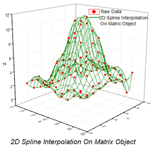
Two-dimensional interpolation/extrapolation can also be performed on data stored in an Origin matrix. Origin supports five methods for interpolation on Matrix: Nearest, Bilinear, Bicubic, Spline, Biquadratic. You can also specify the interpolation output ranges for X and Y.

To Perform 2D Interpolation on Matrix

Activate the matrix that contains your input data.
Select Analysis: Mathematics: 2D Interpolation/Extrapolation from the menu. This opens the minterp2 dialog box.
Choose your input options and click OK. The minterp2 X-Function is called to complete the calculation.

Dialog Options for 2D Interpolation on Matrix

Recalculate	Controls recalculation of analysis results None Auto Manual For more information, see: Recalculating Analysis Results
Input Matrix	Specify the matrix that contains the data to be interpolated/extrapolated. For help with range controls, see: Specifying Your Input Data
Method	Specify the interpolation/extrapolation method. Nearest Interpolate using the nearest points. Bilinear Two dimensional linear interpolation. Bicubic Convolution Two dimensional interpolation using bicubic convolution. Spline Two dimensional spline interpolation. Biquadratic Two dimensional quadratic interpolation. Bicubic Lagrange Two dimensional interpolation using Lagrange polynomials.
Number of Cols	The number of columns in the output matrix.
Number of Rows	The number of rows in the output matrix.
Missing Value Pretreatment	Specify the method to preprocess missing values in 2D interpolation Skip Remove all missing values first and then run interpolation. Interpolated with Renka Cline Renka Cline: For an arbitrary point P, compute the interpolated value using the data values and gradient estimates at each of the three vertices of the triangle which contains P.
Coordinates	Specify the coordinates/XY mapping of the output matrix. First X The first x value of the output matrix. Last X The first x value of the output matrix. First Y The first y value of the output matrix. Last Y The last y value of the output matrix.
Output Matrix	Specify the output matrix for the interpolated/extrapolated data.

Algorithm for Interpolation on Matrix

Nearest (neighbor) interpolation:

Calculate the interpolated value using the nearest grid points.

Polynomial interpolation:

This type of interpolation includes Bilinear, Biquadratic, Bicubic Convolution and Bicubic Lagrange methods, all of which operate similarly. For instance, to calculate the value at point $P(x,y)\!$ by the biquadratic interpolation method, we first perform 1D quadratic interpolation vertically, based on data points $P_{(i,i)}\!$ , $P_{(i,i+1)}\!$ , $P_{(i,i+2)}\!$ to generate $p_i^{\prime }$ , which has the same $y\!$ value as $P\!$ . Then we calculate $P_{i+1}^{\prime }$ , and $P_{i+2}^{\prime }$ . Values $P_{i}^{\prime }$ , $p_{i+1}^{\prime }$ and $p_{i+2}^{\prime }$ define a line through $P\!$ . We then perform 1D quadratic interpolation horizontally to evaluate the value at $P\!$ .

The difference between Bilinear, Biquadratic, Bicubic Convolution and Bicubic Lagrange methods is in the use of different order polynomial functions. The interpolating polynomial of order n-1 through n points is:

$P(x) = \cfrac{(x-x_1)(x-x_2)\cdots (x-x_{n-1})}{(x_0-x_1)(x_0-x_2)\cdots (x_0-x_{n-1})}y_0$ $+\cfrac{(x-x_1)(x-x_2)\cdots (x-x_{n-1})}{(x_1-x_1)(x_1-x_2)\cdots (x_1-x_{n-1})}y_1+ \cdots$ $+ \cfrac{(x-x_1)(x-x_2)\cdots (x-x_{n-1})}{(x_{n-1}-x_1)(x_{n-1}-x_2)\cdots (x_{n-1}-x_{n-1})}y_{n-1}$

Spline interpolation:

References

- Willian H. Press, etc. Numerical Recipes in C++, 2nd Edition. Cambridge University Press. (2002)