4.5.1.1 Set Column/Cell Values

SetColVal

Set Column Values Setting Column Values Worksheet Set Column Values to Reference Other Info Use Spreadsheet Notation to Set Column Values Cell Formula Formula Bar Set Multiple Column Values

Using Metadata in Worksheet in Calculation – Part 1: Column Label Rows New in Origin 2021- The Formula Bar Extracting Dates from Text Strings How to Create a Timeline in Origin

Summary

Origin provides several ways to compute a column or matrix of values. One of Origin's most powerful features is Set Column Values, a tool for performing mathematical operations, generally on values stored in a workbook or matrix. These operations can make use of Origin's built-in functions, custom Origin C functions, Python functions, mathematical and logical operators, built-in or user-defined variables, and can even allow for pre-processing of input data.

This tutorial will show you how to compute cell or column values by:

• Filling a Column with an Arithmetic Series
• Using Built-in Functions
• Using Other Columns of Values
• Using Cell Values
• Using Variables from Workbook Metadata

In addition, you will learn:

• How to enter a formula into worksheet cell to compute cell values
• Auto behaviors of setting cell values

Setting Column values

Filling a Column with Arithmetic Series

Origin provides multiple methods to fill a column with arithmetic series.

Using Auto Fill

1. Enter a few starting values in cells.

   

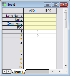
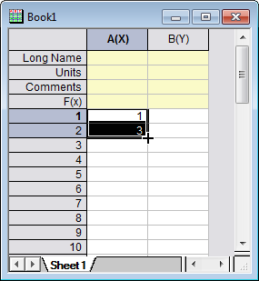
2. Select the two cells.
3. Move the mouse to the bottom right-hand corner of the second cell. The cursor will change to display "+".

   

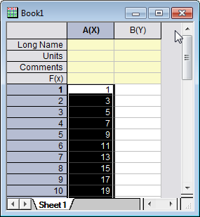
4. Drag the mouse toward the bottom of the column. The column will be filled with 1, 3, 5, 7, ... .

   

Note that a row can also be auto filled by dragging towards the right. In addition, to copy a sequence of cell values to other column or row cells, press SHIFT while selecting the desired sequence, then press CTRL and drag.

Using Filling A Set of Numbers

1. Right click on the column B and select Fill Column with: A Set of Numbers from the context menu to bring up the PatternN dialog
2. Enter 1 in the From edit box and 23 in the To edit box. Enter 2 in the Increment edit box

   

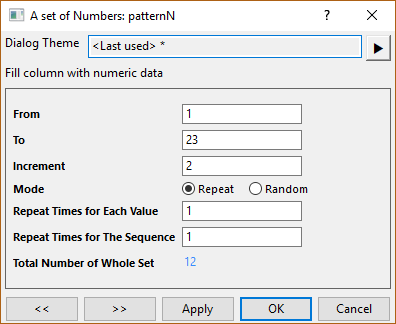
3. After you click the OK button, Column B will be filled with values: 1, 3, 5, 7, ...., 23

Using Other Columns

We will show you how to enter expressions in the F(x) row to set column values.

1. Create a new workbook. Import US Metropolitan Area Population.dat from the \Samples\Data Manipulation\ folder.
2. Add a new column to the worksheet (right-click to the right of the last column in the worksheet and select Add New Column from the context menu). Change the Long Name of the column to Population/Sq. Mi.
3. To calculate the population density, enter the expression, A/B, in the F(x) row of column E.

   

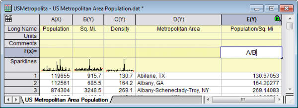
4. The column will get computed using data from the other two columns.

Using Built-in Functions

1. Create a new workbook. Import Step Signal with Random Noise.dat from the \Samples\Signal Processing\ folder.We are going to calculate the moving average of column B, that is, calculating the adjacent average value at each point of column B.
2. Click the Add New Columns button on the Standard toolbar to add a new column C. Highlight this column and right-click, and then click Set Column Values... to open the Set Values dialog.
3. In Set Values dialog, click the Search and Insert Functions button to search for keyword adjacent average.
   
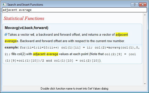
4. Double click function name Movavg(vd,back,forward) to insert it into dialog and close the dialog.
   
5. Highlight the characters vd. replace vd with B, replace back with 0 and replace forward with 2. Your formula should look like this:
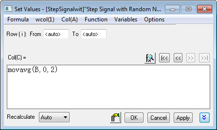
6. Click OK. The last column will fill with the moving average from column B.
   

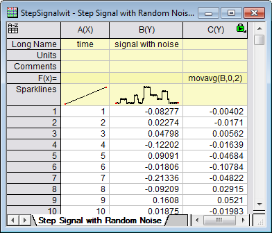
When referring to another column in the same worksheet, you can use index (e.g. "col(1)"), short name (e.g. "A" or "col(A)"), or long name (e.g. "signal with noise") to identify the column.

Using Columns from Other Sheets

The Set Values dialog provides an Variable menu to easily insert range variables that point to columns in other books/sheets, which can then be used to compute column values for the current column.

1. Open the project \Samples\Data Manipulation\Setting Column Values.opj and click on the Columns from Other Sheets subfolder.
2. In the workbook, right-click on the worksheet tab labelled Sample and select Duplicate Without Data. Rename(by double-clicking on the current name) the new sheet as: Corrected Sample.
3. Now you will fill these three columns with data based on formulas that reference columns in the other sheets. Highlight the first column and right-click on it to select Set Columns Values to open the dialog. Select Variables: Add Range Variable by Selection to open the Select from Worksheet dialog. With this dialog, you could select a column from worksheet and insert it as a range variable to the Before Formula Script panel.
4. When the Select from Worksheet dialog is open, activate the Sample sheet, highlight column A to select and click the button to confirm selection and click OK (accept Column Notation) in the Insert Mode dialog box that appears.
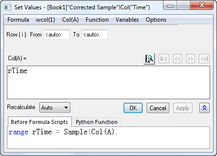
5. "range r1 = Sample!Col(A);" will be automatically inserted into the Before Formula Scripts panel. Edit the formula to read as:

   range rTime = Sample!Col(A);

6. Then enter rTime in the Column Formula and click the OK button to generate data for the first column and close the dialog.
   
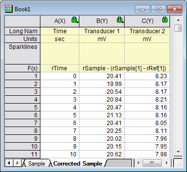
7. In the Corrected Sample worksheet, highlight column B and column C and right-click on them. From the shortcut menu, select Set Multiple Column Values to open the dialog. Select Variables: Add Range Variable by Selection and insert two range variables, one by one, to the Before Formula Script panel similarly as the previous steps. Edit these new entries as follows:

   range rSample = Sample!Col(B);

   and

   range rRef = Reference!Col(B);

8. Now we will edit the range variables in the Before Formula Scripts panel and use another expression to get the same results. Remove the column names Col(B) of the two range variables and select Variables: Predefined Variables: wcol(j) in both lines so it looks as follows:

   range rSample = Sample!wcol(j);

   range rRef = Reference!wcol(j);

9. Then input the following expression into the Column Formula:

   rSample - (rSample[1] - rRef[1])

   

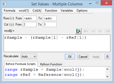
10. Click the OK button to generate data for the column B and column C of the Corrected Sample worksheet.
    

You reference a particular cell value with square brackets, so [1] in the Column Formula expression above means the first element. You can select Formula: Save and Formula: Load in the Set Column Values dialog to save your formulas and reload them into other columns to generate new data.

Using Cell Values

Values contained in specific worksheet cells can be referenced and used to compute the formula for setting column values. This provides an easy way to use worksheet cells as control cells for updating values in a column.

1. Open the project \Samples\Data Manipulation\Setting Column Values.opj and switch to the Cells in a Worksheet subfolder in Project Explorer.
2. Right-click on column C and select the Set Column Values... context menu to bring up the Set Values dialog.
3. Use the Variables: Add Range Variable by Selection menu item to open the Select from Worksheet dialog. Then select column G(Value) in this worksheet, click the button.
   Click OK when the Insert Mode dialog appears (accept Column Notation) to add its expression to the Before Formula Scripts panel.
4. In the Before Formula Scripts panel, change the name of the range variable to be rControl and add these additional lines so that the script looks like below

   range rControl = Col(G);
   //range r1 = Col(7);
   int nOrder = rControl[2];
   int nPoints = rControl[3];
   differentiate -se iy:=(1,2) order:=1 smooth:=1 poly:=nOrder npts:=nPoints 
   oy:=(1,3);

   The script calls the differentiate X-Function and passes the cell values from column G as arguments for polynomial order and number of points, which controls the Savitzky-Golay smoothing performed during the differentiation.
5. The Set Values dialog then should be as following:
   
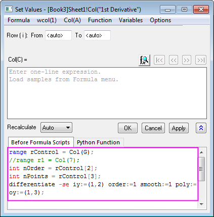
6. Click OK to close the dialog and see the results in column C. Now you can try to change the values in column G, to change the output.

Note: Allowed values of polynomial order are 1 to 9.

The graph shown in the worksheet was first created and then embedded into the worksheet by merging a group of cells.

Using Variables from Workbook Metadata

Metadata stored in the workbook, such as variables saved when importing data using the Import Wizard, can be referenced and used for computing column values.

1. Open or continue working with \Samples\Data Manipulation\Setting Column Values.OPJ, and switch to the Worksheet Metadata subfolder from the Project Explorer window.
2. Select column A and right-click to select the Insert menu option. A new column is inserted to the left of column A.
3. Select the first column (this newly inserted column) and right-click on it. Then select the Set Column Values menu item to open the Set Values dialog.
4. Select the Variables: Add Info Variable menu item to open the Insert Variables dialog. Select Numeric int from the Variable Type drop-down list. Expand the USER.VARIABLES node and click to highlight NUMBEROFPOINTS row with Value as 3800. Press the Insert button to insert this variable into the Before Formula Scripts panel.
   
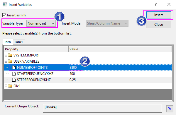
5. Next, set Variable Type to Numeric double. Hold the Shift key down to select both StartFrequencyKHz and StepFrequencyKHz, and then press Insert to insert these two variables. Press the Close button to close the dialog.
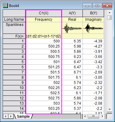
6. In the upper Column Formula panel, input {d1:d2:d1+(n1-1)*d2} and then press the OK button to generate data and close the dialog. The column will be filled with frequency values.
7. Highlight the first and second columns, right-click on them and select Set As: XYY to change the plotting designations to X and Y. After you change the long name of the first column to Frequency, the worksheet should look like:
   

Setting Cell Values

In the Cell-Edit Mode, you can enter a cell formula beginning with an equals sign "=" into a cell (a data cell or UserDefined Parameter Row cell) just as below.

Once the formula has been entered, you exit edit mode (in-place edit or Edit: Edit Mode) to see the resulting cell value.

Let us use an example to show you how cell formulas work in Origin:

1. Open a new workbook in your Origin Project.
2. Import the sample data "automobile2.dat" located at the folder <Origin Program Folder>Samples\Statistics into the workbook.
   
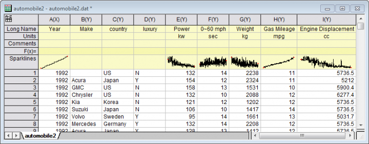
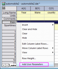
3. Right-click on the header cell of column label row "F(x)=" and select Add User Parameters from the context menu to add a user parameter.
   
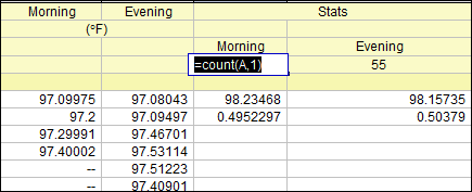
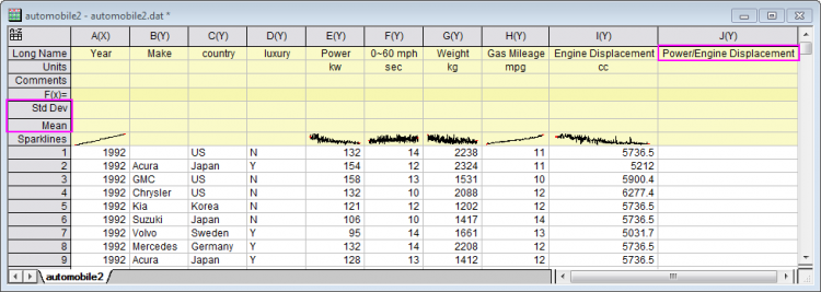
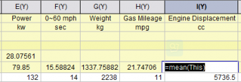
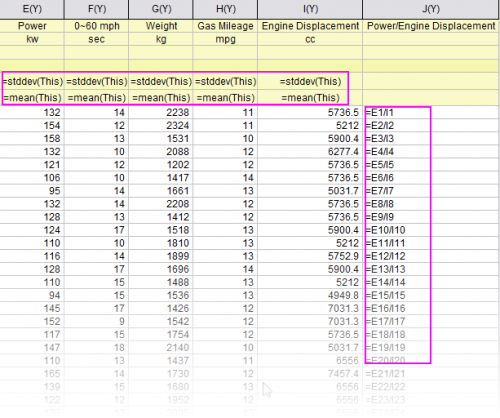
4. Here, let's add two user parameters and enter Mean and Std Dev as their parameter names separately. And then, add one more column at the end of this worksheet, enter Power/Engine Displacement as the column Long Name.
   
5. Select Edit: Edit Mode menu to switch to the Edit Mode. And then, in the cell Mean and Std Dev of Col("Power"), enter =mean(this) and =stddev(this) respectively. Once the edit done, click outside the cell to exit cell-edit mode reselect the Edit: Edit Mode menu item to display cell formula results.
   

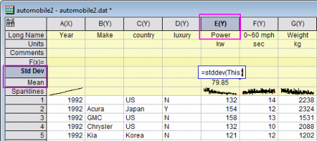
   Note: About the meaning of the variable "This", please refer to this page.

6. Click the cell Mean of Col("Power") to select it, put the cursor to the lower right corner of this cell. When the cursor turns to a cross +, grab this "+" handle and drag with your mouse horizontally to Col("Engine Displacement"). Release the cursor, you will found other cells of this row will be filled with some result values. Alternately, you could simply double-click on the "+" handle and copy the formula to all Mean row cells to the right of Col("Power").
   
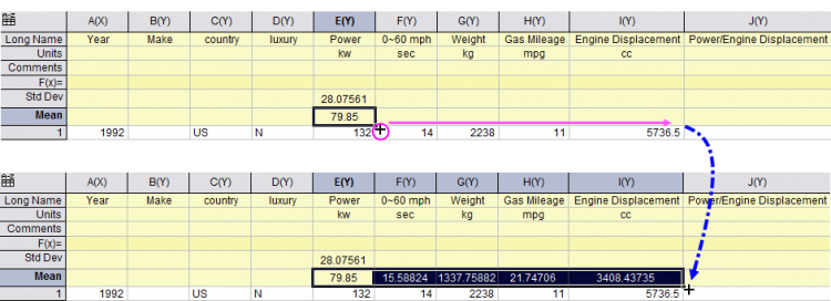
7. Double-click those Mean cells, you will found the filled formulas are all same, =mean(this).
   
8. Do the same thing for the Std Dev row to calculate the standard deviation for all these five columns.
9. Go to the last column we just added, in the first cell enter =E1/I1.
   

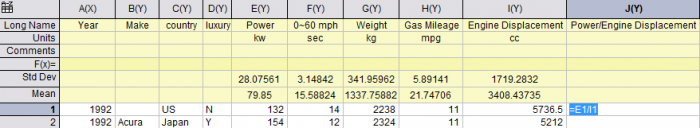
   Note: Here, E1 means the first cell of col(E) and I1 means the first cell of col(I). You can refer to this page to learn more about the formula.

10. Release your cursor to execute the division. Use the same way at Step 6 to grab this "+" handle and drag with your mouse vertically to the end cell of this column (Hint: If you hover on the lower-right corner of the cell, directly over the cell handle, the cursor changes to a "+" sign. When this "+" sign appears, double-click to extend the formula to the end of the column. This is faster and easier than dragging with your mouse).
    
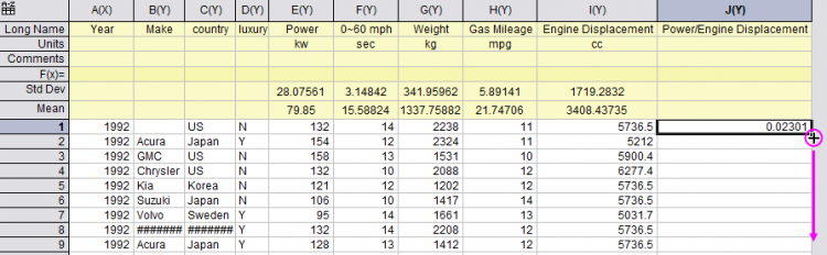
11. Release the cursor to get all division results of col(E)/col(I) at each row.
    

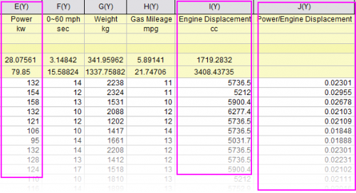
Select Edit: Edit Mode menu, you can check and edit all these cell formulas.