4.5.2.3 Data FilterData-Filter
Summary
The Data Filter is a column-based tool to reduce rows of worksheet data, and consequently also hide the undesired rows for relevant data analysis and graphing. Three data formats are supported: numeric, text and date/time.
Minimum Origin Version Required: Origin 2015 SR0
What you will learn
This tutorial will show you how to:
- Use the data filter to reduce worksheet data
- Auto update the graphs and analysis results when apply a column filter
- Add a floating graph to a worksheet.
Steps
- Start with an new workbook. Select Help: Open Folder: Sample Folder... to open the "Samples" folder. In this folder, open the Statistics subfolder and find the file automobile.dat. Drag-and-drop this file into the empty worksheet to import it.
- Highlight column C(Power), right click and choose Set As:X in the context menu to set this column as X.
- Highlight column C and G (hold Ctrl key when clicking), click the
 button on the 2D Graph toolbar to generate a scatter plot from these two columns. button on the 2D Graph toolbar to generate a scatter plot from these two columns.
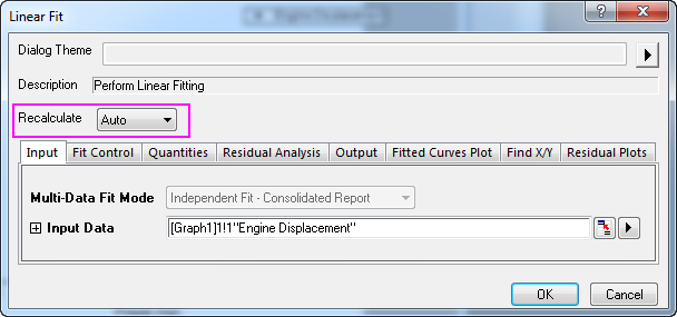
- Activate the generated graph and select Analysis:Fitting:Linear Fit from menu item to open the Linear Fit dialog. In this dialog, set Recalculate to Auto to ensure auto update of the analysis result, accept other settings as default and click OK to carry out the analysis.
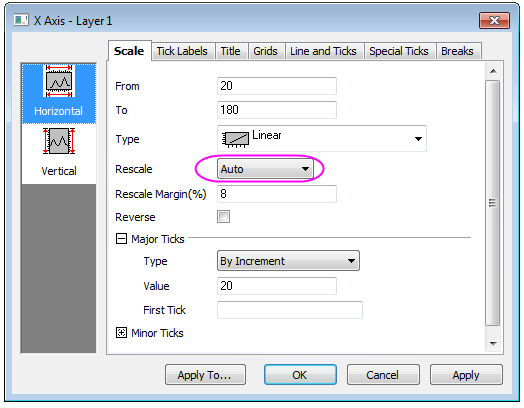
- A fitted curve and a result table will be added to the graph. Activate the graph again and double click on the X axis to open the Axis dialog. Select the Horizontal icon in the Scale tab, then choose Auto for Rescale. Do the same for the Y axis (Vertical icon) and also set its rescale mode to Auto. Click OK to apply the settings and close the dialog.
- Go back to the original worksheet automobile and click Column: Add New Columns and add 7 columns to the worksheet.
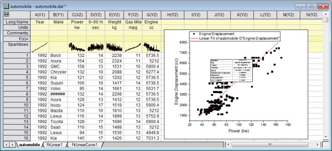
- Right-click in the gray area to the right side of the worksheet columns and select Add Graph... in the context menu to open the Graph Browser. In this dialog, select the previously generated graph in the left panel and click OK to add this graph as a floating chart to the worksheet. Drag the floating chart onto the empty worksheet columns you just created and resize it using the selection handles.
- Highlight column A and B and click the Add/Remove Data Filter button
 on the Worksheet Data toolbar to add empty data filters to both columns. on the Worksheet Data toolbar to add empty data filters to both columns.
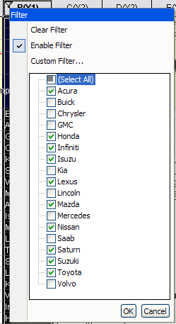
- Click the Filter icon
 on the column header of column B, clear the check boxes before Buick, Chrysler, GMC, Kia, Lincoln, Mercedes, Saab, Volvo to hide all rows with these entries, to leave only the Japanese makers. Click OK to apply the filter. The worksheet data, graph and analysis result will all be auto updated accordingly. on the column header of column B, clear the check boxes before Buick, Chrysler, GMC, Kia, Lincoln, Mercedes, Saab, Volvo to hide all rows with these entries, to leave only the Japanese makers. Click OK to apply the filter. The worksheet data, graph and analysis result will all be auto updated accordingly.
- Click the Filter icon on the column header of column A and select Between, note that the data type of column A is numeric by default from importing. Accept default setting of the Between dialog and click OK. A data filter is applied to this column.
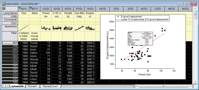
- Again click the Filter icon on column A and this time choose Custom Filter in the context menu to customize the filter, change the Condition as x.between(1996,2000) to set the From and To value respectively, click the Test button and in the original worksheet, only the rows meet this testing condition will be highlighted, this works as a preview of the data reduction.
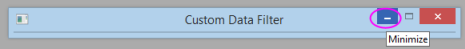
 | To view the whole worksheet at this stage, you can minimize the Custom Filter dialog, allowing you to scroll up and down the worksheet freely. You can later restore the dialog by clicking the "Minimize" button.
|
- Click the OK button to apply the new filtering condition and the data, graphs and analysis results are updated and the graph is also auto rescaled.
| Beginning with Origin 2019, you can copy data filters from one column and paste to other columns of data. Right-click on the column's Filter cell and choose Copy; or click on the Filter cell and press Ctrl+C to copy the filter. Select your target column(s) and press Ctrl+V to paste the filter and apply it to data in those columns.
|
|