4.5.3 Pivot TablePivot-Table
Summary
The Pivot Table provides a quick way to summarize your data, and to analyze, compare, and detect relationships in your data. This tool can sort, count, sum, or compute minimum, maximum, or mean of data stored in a worksheet.
Minimum Origin Version Required: Origin 2015 SR0
What you will learn
- How to summarize data by a Pivot Table.
- How to sort output by row or column totals in Pivot Table.
- How to combine small values in columns or rows, and custom extra value.
Import Data from Database
- Before creating a pivot table, we should can import data from database.
Suppose we have already set up a database named AdventureWorks2008R2 on a server machine - myServer - running SQL Server, with user name as "accounting", and password as "mydatabase".
- To connect the database, we use a connection string:
Provider=SQLOLEDB.1;Password=mydatabase;Persist Security Info=True;
User ID=accounting;Initial Catalog=AdventureWorks2008R2;Data Source=myServer
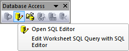
- Activate an empty worksheet and open SQL Editor by clicking the Open SQL Editor button on the Database Access toolbar.
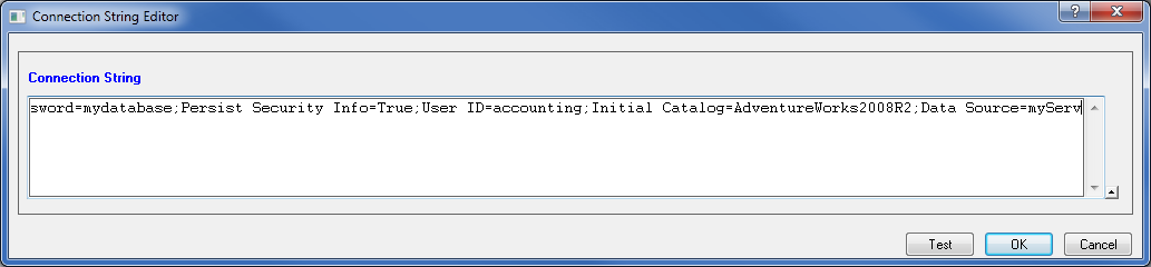
- Select menu item Edit Connection String... from SQL Editor's File menu, in the open dialog, put the connection string (see step 1 above) to the text box. And then you can click the Test button to test if the connection is fine. If fine, click the OK button to connection to the database.
- In the right text box, put the following SQL statements.
SELECT
DatePart(yyyy, SOH.OrderDate) AS YEAR,
CR.Name As CustomerCountry,
	Pr.Name As ProductName,
	Pr.Color As ProductColor,
	PC.Name As ProductCategory,
	PS.Name As ProductSubcategory,
	SOH.OrderDate As OrderDate,
	SOD.OrderQty As OrderAmount,
	SOD.LineTotal As TotalCost
FROM Person.CountryRegion AS CR
INNER JOIN Person.StateProvince AS SP
ON SP.CountryRegionCode = CR.CountryRegionCode
INNER JOIN Person.Address AS A
ON A.StateProvinceID = SP.StateProvinceID
INNER JOIN Person.BusinessEntityAddress AS BEA
ON BEA.AddressID = A.AddressID
INNER JOIN Person.Person AS P
ON P.BusinessEntityID = BEA.BusinessEntityID
INNER JOIN Sales.PersonCreditCard AS PCC
ON PCC.BusinessEntityID = P.BusinessEntityID
INNER JOIN Sales.SalesOrderHeader AS SOH
ON SOH.CreditCardID = PCC.CreditCardID
INNER JOIN Sales.SalesOrderDetail AS SOD
ON SOD.SalesOrderID = SOH.SalesOrderID
INNER JOIN Production.Product AS Pr
ON Pr.ProductID = SOD.ProductID
INNER JOIN Production.ProductSubcategory AS PS
ON PS.ProductSubcategoryID = Pr.ProductSubcategoryID
INNER JOIN Production.ProductCategory AS PC
ON PC.ProductCategoryID = PS.ProductCategoryID
--WHERE SOH.OrderDate BETWEEN '1/1/2005' AND '12/31/2008'
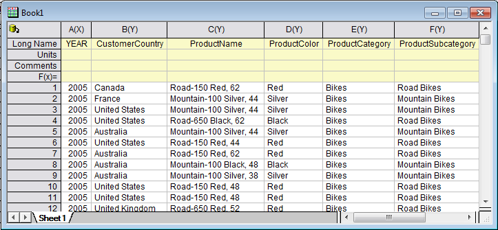
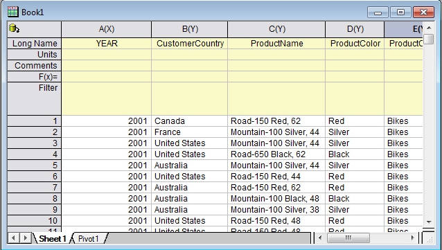
- Select menu File: Save to Active Worksheet to save these settings to the worksheet, and then select menu Query: Import to import the data into worksheet, and then close SQL Editor. We can see the imported data form the image below.
- Click Close to close the dialog.
Create a Pivot Table
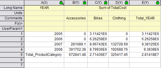
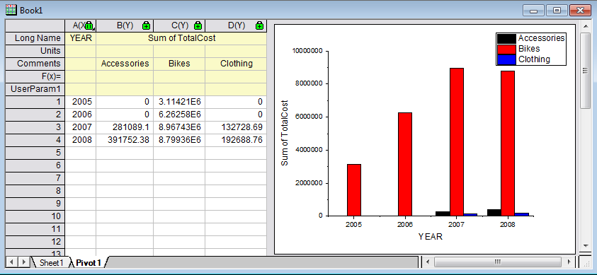
The imported dataset is a total cost summary of three product categories(Bikes,Accessories, Clothing) in six different countries by year. Suppose now you want to create a pivot table to see the yearly Sum of Total Cost of different product category. Follow the steps below to create the pivot table.
- Activate the Sheet1, select Restructure: Pivot Table from the main menu to open the dialog. And specify the following settings in the dialog:
- For Pivot Table Row Source, click the triangle button
 to add column A. to add column A.
- For Pivot Table Column Source, click the triangle button to add column E.
- Select Sum with the Summarize by drop-down list. Then select column I for Pivot Table Data Source.
- Expanding Options branch, check Total for Rows and Total for Columns check boxes, and select Row Label Ascending from the Sort Output Rows drop-down list.
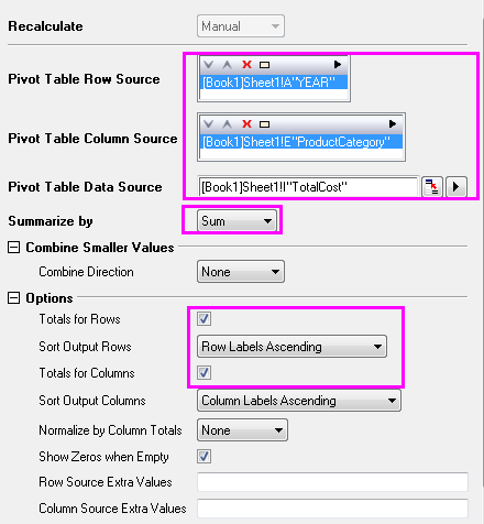
- Click the OK button to create the pivot table. The table should like this:
Combine Small Values
In this section, we will show you how to present those categories with the percentage of the summarized value (Count/Sum/Mean/Min/Max) accounts for that of grand total exceeding a threshold percent, and combine small value categories into a default Others category.
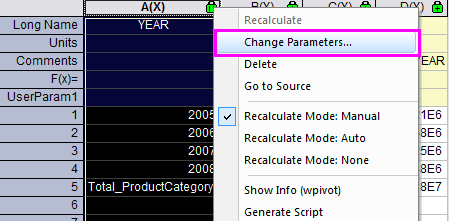
- Based on the above example, click on the lock icon in the Pivot1 worksheet, and select Change Parameters to open the dialog again.
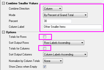
- Specify the following settings in the dialog:
- Expanding Combine Smaller Values branch, select Column in the Combine Direction drop-down list,
- Select By Percent of Grand Total in Mode drop-down list.
- Enter 30 in Percent textbox and Other Smaller Items in the Column Label textbox.
- Expanding Options branch, uncheck the boxes of Totals for Rows and Totals for Columns
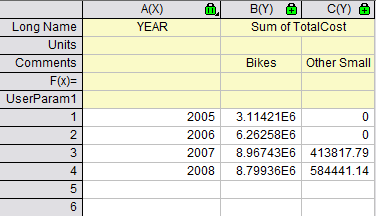
- Click OK button. The pivot table shows the summarization of data by Sum. And only Category Bikes has the percent of grand total exceeding the threshod percent 30 %, other smaller categories has been reduced into Category Other Smaller Items.
Extra Categories Source
In this section, we will show you how to present those categories that are missing in the source data sheet with ' Column Source Extra Value. This is useful when you want to ensure all needed categories will be presented in the result pivot table that might be used for later plotting.
Suppose we want to know the Sum of Total Cost of different product categories before Year 2007. Follow the steps below to create the pivot table.
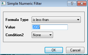
- To filter the years before 2007, we use the data filter. Go to Sheet 1 and select Col A. Click
 button in the main menu bar. Click again the filter icon on Col A and select Less Than. Customize the pop-out filter dialog as follow, then click OK to close the dialog. button in the main menu bar. Click again the filter icon on Col A and select Less Than. Customize the pop-out filter dialog as follow, then click OK to close the dialog.
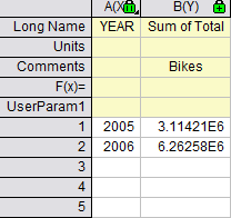
- Click on the lock icon in the Pivot1 worksheet, and select Recalculate. As shown in the following pivot table, only Bikes is presented here, because other two product categories do not has any cost data record in Year 2005 and 2006.
- Back to Pivot1 worksheet, select col(b) and then click Plot > 2D: Bar: Column to plot a column graph(Graph1).
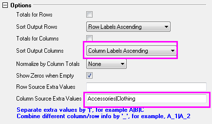
- Next we want to add two missing categories back into the pivot table. Click on the lock icon in the Pivot1 worksheet, and select Change Parameters. Customize the dialog as follow, click OK to close the dialog.
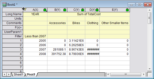
The pivot table would look as follow.
The pivot table would look as follow.
- Back to Pivot1 worksheet again. Click again the filter icon on Col A and select Clear Filter from the pop-up menu to remove the filter. Then select all columns to plot a column graph(Graph2). The graph would show the missing categories.
- Back to Pivot1 worksheet again, right click the grey area and select Add Graph to add Graph2 onto the Pivot1 worksheet
 | Year filtering can also be obtained in Database. In this case, you can customize the favorable time period by rewriting this script:
--WHERE SOH.OrderDate BETWEEN '1/1/2005' AND '12/31/2008'
|
Create analysis template
In this section we will show you how to create analysis template for the pivot table, reimport data from database and reuse the analysis template to create pivot table for new data.
- Activate the Book1, click File: Save Workbook as template and save it as SumTotalCost.ogw.
- Open a new OPJ file and then click File: Open to open SumTotalCost.ogw.
- To change the data source as AdventureWorks2008 in database,
- Activate Sheet1 and open SQL Editor by clicking the Open SQL Editor button
 . .
- Click File: Edit Connection String then type the following string in the open dialog, click Test then click OK to connect the database.
Provider=SQLOLEDB.1;Password=mydatabase;Persist Security Info=True;
User ID=accounting;Initial Catalog=AdventureWorks2008;Data Source=myServer
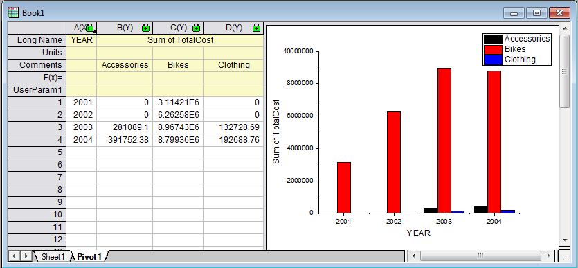
- Back to the SQL Editor dialog, On the right panel, rewrite the last script as
--WHERE SOH.OrderDate BETWEEN '1/1/2001' AND '12/31/2004'
- Select menu File: Save to Active Worksheet to save these settings to the worksheet, and then select menu Query: Import to import the data into worksheet, and then close SQL Editor. We can see the imported data form the image below.
- To update the pivot table, go to Sheet'Pivot1 , click the yellow lock and select Recalculate. The pivot table would be updated according to new data.
- To update the embedded graph,
- double click the embedded graph and a floating chart would pop up.
- Select the graph and click Rescale button to refresh
 . The floating chart would be updated too. . The floating chart would be updated too.
- click the arrow button at the upper right corner of the floating chart to put it back to the worksheet. The worksheet would look as follow.
|