4.6.3 Creating a Custom Report SheetCreate-Custom-Report
Summary
Worksheets in Origin can be customized by merging cells and coalescing various objects such as graphs, external images, links to variables and tables/cells in other sheets, into a custom report.
This tutorial will show you how to add a custom report to an existing analysis template. You can then import new data, recalculate results, and export or print the custom report.
Minimum Origin Version Required: Origin 9.0 SR0
What you will learn
- How to create a custom report sheet
- How to save a custom report as part of an Analysis Template (OGW) and re-use it with new data
Steps
Note: Please complete the previous tutorial named "Creating and Using Analysis Templates" in which an analysis template named MySensorData.OGWU is created.
Importing Data
- Using the File:Open menu item, set the Files of type drop-down to Workbooks (*.ogwu), then navigate to and open the Analysis Template MySensorData.OGWU. This analysis template was saved with a linear fit analysis for column B of the first worksheet, and a customized embedded graph with the data and the linear fit line (note that templates do not contain data, so at this point, you see no data and no results).
- Make the Data worksheet active. Select Help: Open Folder: Sample Folder... to open the "Samples" folder. In this folder, open the Curve Fitting subfolder and find the file Sensor01.dat. Drag-and-drop this file into the worksheet Data to import it.
Creating a Custom Report Sheet
- Right-click on the Data worksheet and select Add to add a new worksheet. Rename this worksheet as Custom Report.
- Activate the Custom Report sheet and choose Format:Worksheet (or hit F4) to open the Worksheet Properties dialog. Go to the Size tab and under the Size node, set Row Number as 20 and Column Number as 9. Then go to the Miscellaneous tab and check the Auto Add Rows check box. Click OK to apply these settings and close the dialog.
- In the worksheet, click and drag on the row headers for Long Name, Unit, Comments and F(x)= to select these four rows. Then right click and select Hide from the context menu. This hides the four rows from the worksheet.
- Highlight the range of the cells in the first three rows for all columns and click the Merge Cells button
 located in the Styles toolbar to merge the cells. Enter the text Sensor Data Analysis Report in this merged cell. located in the Styles toolbar to merge the cells. Enter the text Sensor Data Analysis Report in this merged cell.
- In the 5th row, merge the cells in columns G and H. Repeat for the 6th row. In row 5, column F, enter the text File Name: In row 6, column F, enter the text File Date:.
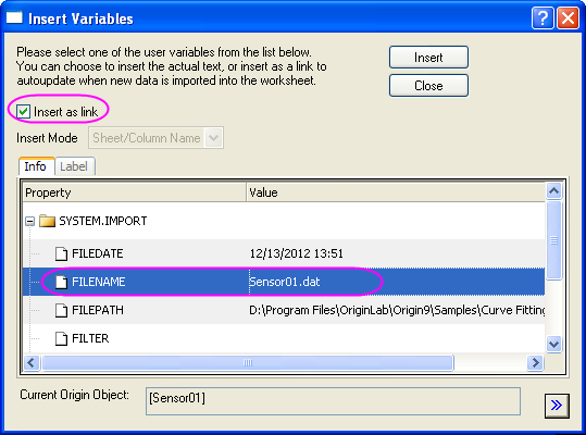
- Right click the merged (column G and H) cells in row 5 and choose Insert Variables from the context menu. Make sure the dialog settings look like those in the image below and insert the FILENAME variable into this cell.
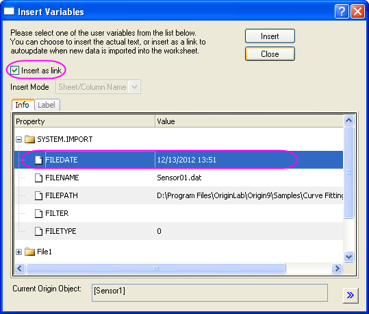
- Right click the merged (column G and H) cells in row 6 and choose Insert Variables from the context menu. Insert the FILEDATE variable following the settings in the image below:
- Right click on the cell containing the date information and choose Format Cells from the context menu. Change the Format drop-down to Date and click OK.
- Go to the FitLinear1 worksheet and locate the Parameters table. Click the triangle button next to it and choose Copy Table from the fly-out menu.
- Go to the Custom Report sheet and select the 9th row in column E. Right click and choose Paste Link. Clear the pasted text Sensor Output in column E by pressing the Delete key.
- In the 13th row, merge the cells in columns G and H. Do the same in the 14th row.
- Return to the FitLinear1 sheet and in the Statistics table, select the two data cells for Pearson's r and Adj. R-Square. Right click and choose Copy to copy only these two cells.
- Go to the Custom Report sheet and select the merged cell in the 13th row, then right-click and choose Paste Link. The two merged cells are filled with corresponding values. Enter the text Pearson's r and Adj. R-Square in the cells to the left of these pasted values.
- In the 8th row, merge the three cells in columns F, G and H. Do the same in rows 12 and 20. Enter the text Fit Parameters, Fit Statistics and Report Date: $(@D, D1) in rows 8, 12 and 20, respectively.
- Right click on the merged cells in row 20 and choose Set Data Style:Rich Text from the context menu. By enabling rich text, the string $(@D,D1) will display as the actual system date.
- Hold the CTRL key and select all cells with numeric values, then right-click and choose Format Cells in context menu, then choose Set Decimal Places= from the Digits drop-down menu, and enter 3 as Decimal Number, and press OK.
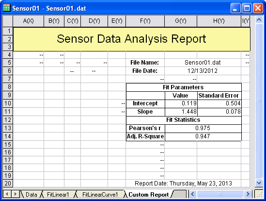
- Using buttons in the Style and Format toolbars, change cell borders, font sizes, styles and colors to customize the report as in the image below below. You may also need to manually adjust the width of some columns to ensure that all text is displayed.
- Go to the FitLinear1 sheet and double-click on the graph under Fitted Curves Plot to open the embedded graph. Right click on the graph's title bar and choose Duplicate from the context menu to duplicate the graph window (Graph1). Double click on the axis of duplicated graph to bring up Axis dialog. Go to Scale tab under both X Axis and Y Axis and choose Auto from the Rescale drop-down list. Then close the original embedded graph window.
- Return to the Custom Report worksheet, right click on the gray area of this worksheet and select Add Graph from context menu. In the Graph Browser, select Graph1 which was created by duplicating the embedded graph. Click OK to add this graph to this worksheet as a floating chart.
- You can manually resize and move this floating chart using its anchor points and position it anywhere in the worksheet.
- Go to Format:Worksheet (or press F4) to open the Worksheet Properties dialog. In the View tab, under the Show Grid Lines node, clear the check boxes next to Column Grid and Row Grid. On the Format tab, make sure Apply To is set to Data, and select Show Missing as Blank to show missing values as blank instead of displaying the "--" characters. Press OK to close this dialog.
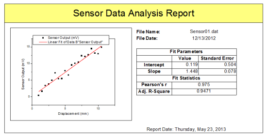
- Select File:Print Preview to preview the custom report. It should look similar to the image below:
 | Beginning with Origin 2018b all merged cells within a selected range, including non-contiguous blocks of merged cells, can be un-merged by clicking the Merge cells button on the Style toolbar.
|
Saving the Analysis Template
- Activate the workbook and select File:Save Workbook as Analysis Template.
- Browse to a desired file path and enter the file name SensorDataReport and click Save.
- You can use this SensorDataReport.OGWU as an Analysis Template for future analyses of similar data, and the custom report will also be included in the workbook.
Re-using the Analysis Template
- Start a new project and then select the menu item File: Recent Books and from the fly-out options select the Analysis Template SensorDataReport.ogw which was saved earlier.
- Make the Data worksheet active, select Help: Open Folder: Sample Folder... to open the "Samples" folder. In this folder, open the Curve Fitting subfolder and find the file Sensor02.dat. Drag-and-drop this file into the worksheet "Data" to import it.
- The linear fit results and the custom report are automatically generated using the newly imported data.
|