5.3.5 Two-Way Mixed-Design ANOVA

2Way-Mixed-Design-ANOVA

Summary

The two-way mixed-design ANOVA is also known as two way split-plot design (SPANOVA). It is ANOVA with one repeated-measures factor and one between-groups factor.

Minimum Origin Version Required: OriginPro 2016 SR0

What you will learn

This tutorial will show you how to:

• Perform the two-way mixed design ANOVA.
• Interpret results of the two-way mixed design ANOVA

User Story

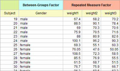
A researcher wants to know whether a treatment can help people lose weight. 48 participants(24 male) take part in the study. The researcher record their weights every three months during the treatment program.

Preparing Analysis Data

To preform two-way mixed-design ANOVA, the data can be arranged as below

Performing Two-Way Mixed-Design ANOVA

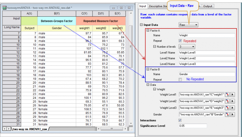
1. Open a new project or a new workbook. Import the data file \Samples\Statistics\ANOVA\two-way rm ANOVA1_raw.dat
2. Select Statistics: ANOVA: Two-Way Repeated Measures ANOVA... from Origin menu
3. In the opened dialog, choose the Input tab,
   • Set Input Data as Raw
   • Expand Factor A branch, change the Name as Weight and set Number of Levels = 3. Expand Factor B branch, change the Name as Gender and unselect Repeat check box
   • In the Data branch, set column C, D and E to be Weight Level1, Weight Level2 and Weight Level3, respectively, and set column B as Gender
   • Select Interactions check box

   

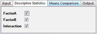
4. Choose the Descriptive Statistics tab. select all check boxes

   

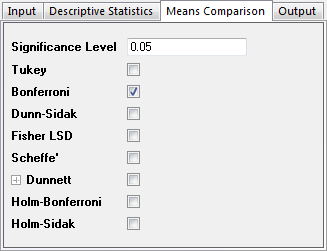
5. Choose the Means Comparison tab, select Bonferroni check box.

   

6. Click OK button to perform the analysis

Interpreting the Results

Go to the worksheet ANOVATwoWayRM1, where the analysis results are listed.

You can refer to this interpreting results help page for details of interpreting results of repeated measures ANOVA. .

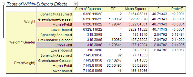
1. From the Mauchly's Test of Sphericity table, we can see Prob>ChiSq(0.01258) < 0.05. So the repeated measure variable, Weight, violates the Sphericity assumption. We should consider the Greenhouse-Geisser correction ect. While the Epsilon is larger than 0.75, we will look at the Huynh and Feldt correction in step 2 below

   

2. From the Tests of Within-Subject Effects table, we can see
   • For Weight, the p_vaule is about 0 in the Prob>F column, It indicates that the weight is a significant effect, that is, the weights change over time.
   • While the interaction, Weight*Gender, is not significant different(p_value = 0.14025), we can conclude that there is not a significant interaction effect, Weight*Gender

   

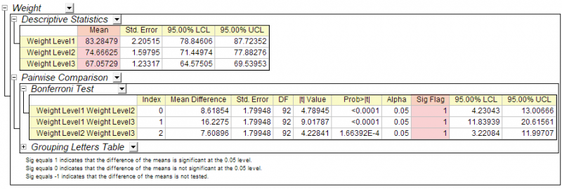
3. We can further study how the weights change over time during the treatment. Expand the Weight branch. From the tables we can see
   • From the Descriptive Statistics table we can see that the weights are decreasing
   • In the Pairwise Comparison table, the 1 in the Sig Flag column indicates the pair of group is significant different. We can draw conclusion that the weights are significantly decreasing

   

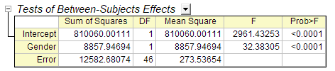
4. From the Tests for Between-Subjects Effects table, we can see Gender is a significant effect, that is, Female and Male can be significant different.

   

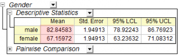
5. Look at the Gender branch to see the details.
   • There are only two levels for Gender and we already know they are significant different, so we don't need to look at the Pairwise Comparison table
   • From the Descriptive Statistics table we can see that average weight of men is more than women.