6 Sample Projects with attached Python Code

1 Samples using Origin Projects
2 How to Execute Python Code from a Button
- 2.1 The Show Code Button

Samples using Origin Projects

This page lists Python examples added in Origin/OrignPro version 2021 that are based on Origin Project files. The Python code file is attached to the project. The projects also have buttons to run the code and to open the code in Code Builder to view, run and debug.

The projects can be found in the \Samples\Python sub folder.

A brief description of each sample and the code associated with the sample are provided below. This will give you an overall idea as to how easy it is to work with the new originpro package for embedded Python in Origin.

Batch Peak Analysis of Multiple Files

In this example, batch peak analysis is performed by importing one data file at a time. Baseline subtraction and peak fitting is performed on the data. The peak parameters are placed on a graph displaying the data and the fit results. The graph is then exported as a png image file.

import originpro as op
import os

path = op.path('e') + "samples\\Batch2\\" 

for file in os.listdir(path): 
    fullpath = os.path.join(path, file)
    wks = op.find_sheet(ref='Book1')
    wks.from_file(fullpath)
    
    op.wait() # wait until operation is done
    op.wait('s', 0.05)#wait further for graph to update
    
    weight = wks.get_label(1,'C') # get column comment for export graph name
    gp = op.find_graph("Graph1")
    graphpath = gp.save_fig(op.path()+f'weight - {weight}.png', width=800)
    print(graphpath)
    
os.startfile(op.path()) # open folder containing exported graphs

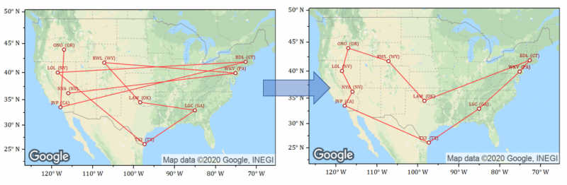
Travelling Salesperson Problem

This example uses scikit-opt package to find optimal solution for the Travelling Salesperson problem. US airport data with latitude and longitude values is used for the destination points. The randomly selected airport locations and the optimized path are displayed in a graph over Google map image.

Code for picking a random set of cities (worksheet rows):

import pandas as pd
import originpro as op
#transfer data from sheet "All Airports" sheet to a DataFrame
#then randomly choose 10 cities to put to sheet name "Selected"
wksSource = op.find_sheet('w', '[Book2]"All Airports"')
df = wksSource.to_df()
#no need to put quotes around sheet name if it has no space
wks = op.find_sheet(ref='[Book2]Selected')
wks.clear()
wks.from_df(df.sample(10))

Code for optimizing distance:

# Python code to solve Travelling Salesperson Problem using scikit_opt
# Optimization code based on the example in this page: https://pypi.org/project/scikit-opt/
    
import sys
import numpy as np
import pandas as pd
import originpro as op
    
# Get to the "Selected" sheet and retrieve data
wks = op.find_sheet(ref='[Book2]Selected')
lat = wks.to_list('LATITUDE')
lon = wks.to_list('LONGITUDE')
coordinates = list(zip(lat, lon))

# Get number of airports/points from column length
num_points = len(coordinates)

from scipy import spatial
distance_matrix = spatial.distance.cdist(coordinates, coordinates, metric='euclidean')
def cal_total_distance(routine):
    '''The objective function. input routine, return total distance.
    cal_total_distance(np.arange(num_points))
    '''
    num_points, = routine.shape
    return sum([distance_matrix[routine[i % num_points], routine[(i + 1) % num_points]] for i in range(num_points)])


# Do optimization
from sko.GA import GA_TSP

ga_tsp = GA_TSP(func=cal_total_distance, n_dim=num_points, size_pop=50, max_iter=500, prob_mut=1)
best_points, best_distance = ga_tsp.run()

# Convert best_points to a list
order=best_points.tolist()

# Loop over to build the row order list
row_order = [0] * num_points
count=0
while (count<num_points):
    row_order[order[count]]=count+1
    count=count+1

# Put the row order into 1st column of the worksheet, sort worksheet by first column
wks.from_list(0, row_order)
wks.sort(0)

# copy first row and append to the end to close the loop on the graph
row1 = wks.to_list2(0,0)
wks.from_list2(row1,num_points)

Logistic Regression

This example performs Logistic Regression Analysis of the data from he worksheet. The parameter values and 95% Confidence Intervals from the analysis are output to a new worksheet. A message is displayed in script window with information on the optimization process.

#This example requires to install statsmodels module

import pandas as pd
import statsmodels.api as sm

import originpro as op

#Send active worksheet data to Python's DataFrame
#Columns C and D in the worksheet are categorical columns 
wks = op.find_sheet( 'w' )
df = wks.to_df()

#Perfrom Logistic Regression in Python
cat_columns = df.select_dtypes(['category']).columns
df[cat_columns] = df[cat_columns].apply(lambda x: x.cat.codes)
df['intercept'] = 1.0

logit = sm.Logit(df['Career_Change'], df[['Age','Salary','Gender','intercept']])

result = logit.fit()

#Merge two DataFrames by index: result.params (Convert Series to DataFrame first) and result.conf_int()
res_df = pd.merge( result.params.to_frame(), result.conf_int(), right_index=True, left_index=True )
res_df.columns = ['Fitted Parameter', '95% CI Lower', '95% CI Upper']

#Send result to a new worksheet in Origin
wksR = op.new_sheet( 'w', 'Logistic Regression Result' )

#Send DataFrame (res_df) to worksheet (wksR)
#res_df includes three columns, and its index is row names, which should also be set to worksheet.

#Send DataFrame values to worksheet, and first column for DataFrame index.
wksR.from_df( res_df, 0, True )

Bayesian Regression

This example demonstrates Bayesian Ridge Regression by calling the BayesianRidge model from the sklearn package.

# This example requires to install sklearn package.

import numpy as np
import pandas as pd
import originpro as op
from sklearn import linear_model


# Find the worksheet ExpGrowth
# and get the 1st and 2nd columns data to X and y respectively
ws = op.find_sheet('w', 'ExpGrowth')
X = np.array(ws.to_list(0))  # Get the first column's data as numpy array
y = np.array(ws.to_list(1)).ravel()  # Get the second column's data as numpy array

# Create BayesianRidge object, with parameters:
# tol=1e-6, tolerance is 1e-6
# fit_intercept=True, to fit with intercept
# compute_score=True, compute the log marginal likelihood at each iteration of the optimization
# alpha_init=1, initial value for alpha of gamma distribution
# lambda_init=1e-3, initial value for lambda of gamma distribution
blr = linear_model.BayesianRidge(tol=1e-6, fit_intercept=True, compute_score=True, alpha_init=1, lambda_init=1e-3)

degree = 10  # Degree for getting Vandermonde matrix

# Expand X to Vandermonde matrix with degree of 10
# then fit the BayesianRidge model
blr.fit(np.vander(X, degree), y)

# Predict y from the same Vandermonde matrix of X, also return standard deviation
ymean, ystd = blr.predict(np.vander(X, degree), return_std=True)

# Find worksheet for output results
wks = op.find_sheet('w', 'Results')

# Output coefficients, because X is expanded with 10 degree of Vandermonde matrix
# so there are 10 coefficients
wks.from_df(pd.DataFrame(blr.coef_, columns=['Coefficients']), 0)

# Output intercept
wks.from_df(pd.DataFrame(np.array([blr.intercept_]), columns=['Intercept']), 1)

# Output alpha and lambda of gamma distribution
wks.from_df(pd.DataFrame(np.c_[['Alpha', 'Lambda'], [blr.alpha_, blr.lambda_]], columns=['Gamma Parameters', 'Gamma Parameter Values']), 2)

# Output score of each interation
wks.from_df(pd.DataFrame(np.c_[np.arange(0, blr.n_iter_+1), blr.scores_], columns=['Iteration', 'Score']), 4)

# Output independent and predicted dependent, and standard deviation
wks.from_df(pd.DataFrame(np.c_[X, ymean, ystd], columns=['Indep', 'Predicted Y', 'STD']), 6)

Friedman's Super Smoother

In this example, data with noise is smoothed using the Friedman's Super Smoother method.

#This example requires to install supersmoother and pandas packages
from supersmoother import SuperSmoother

import originpro as op
import numpy as np
import pandas as pd

#Get data from the active worksheet
wks = op.find_sheet('w')
cx = np.array( wks.to_list( 0 ) )
cy = np.array( wks.to_list( 1 ) )

#Perfrom Friedman's Super Smoother
#alpha: smoothing level, (0 < alpha < 10)
smoother = SuperSmoother( alpha = 2 )

#Fit the smoother
smoother.fit( cx, cy );

#Predict the smoothed function for inpit x
yfit = smoother.predict( cx )

#Output the smoothed result to worksheet in Origin.
df = pd.DataFrame( {'Smoothed': yfit} )
wks.from_df( df, 2 )

Hyperspectral Image Stack and PCA

This example demonstrates how to reduce image stack data using Principal Component Analysis (PCA).

The data is hyperspectral image data over a range of wavelengths, from a MATLAB .mat file. The data size is reduced using PCA but still keeping as much useful information as possible.

import numpy as np
import pandas as pd
import originpro as op
from sklearn.preprocessing import StandardScaler
from sklearn.decomposition import PCA


if __name__ == '__main__':
    # Find matrix sheet named MBook1, this sheet includes 200 matrix objects as image stacks, for 200 bands hyperspectral data
    msX = op.find_sheet('m', 'MBook1')
    
    # Get the 200 bands data from matrix sheet as 3d numpy array
    # dstack=True is to use dstack, so the data is in the shape of (rows, cols, depths)
    # here depths should be 200, mean 200 bands, 
    # rows and cols are number of rows and cols of image for each band
    X = msX.to_np3d(dstack=True)

    # Reshape X to 2d matrix, here is (-1, X.shape[2])
    # -1 means not care the first dimension's size, and X.shape[2] is depths
    # this equals to X = np.reshape(X, (X.shape[0]*X.shape[1], X.shape[2]))
    # after reshape to 2d matrix, one row of matrix has 200 band values
    # that is one pixel of matrix includes 200 values along depth for 200 stacked images
    X = X.reshape((-1, X.shape[2]))
    
    # Find matrix sheet named MBook2
    # this sheet includes the ground truth data with 16 classes (from 1 to 16)
    # and 0 is not a valid class
    msY = op.find_sheet('m', 'MBook2')
    
    # Get the ground truth data from matrix sheet as numpy array
    # and then reshape it as matrix with only one column
    # (-1, 1) means not care the first dimension's size, but with only one column
    mY = msY.to_np3d().reshape((-1, 1))
    
    X = X[mY.ravel() != 0, :]  # Remove the pixels (rows in X) where class is 0 (0 means invalid class)
    
    # The original number of bands is 220
    # but the number of bands in corrected data is 200
    # those bands covering the region of water absorption are [104-108], [150-163], 220
    # so available bands should exclude these 20 bands
    bands = np.append(np.append(np.array(range(1, 104)), np.array(range(109, 150))), np.array(range(164, 220)))

    # Create StandardScaler object, and then fit and transform X data
    # this is for scaling the data to avoid the problem of different scales of the data
    scaledX = StandardScaler().fit_transform(X)
    
    # Create DataFrame using scaled X data
    # by assigning bands as column header
    scaledX = pd.DataFrame(scaledX, columns=bands)  # Though column header is assigned, not very useful here
    
    n_components = 50  # The data have 200 features (waves for one sample), here use 50 to reduce the dimension from 200 to 50
    pca = PCA(n_components=n_components, svd_solver='randomized', whiten=True, random_state=100, copy=True)  # Create PCA object
    
    # Use the pca object to fit and transform the scaledX data
    # now the data has 50 columns, with the same number of rows
    pcaX = pca.fit_transform(scaledX)

    # Print the sum of percentage of variance explained by each of the 50 components
    print(np.sum(pca.explained_variance_ratio_))

    ws = op.new_sheet('w')  # Create worksheet for output data
    
    # Create DataFrame using the PCA result data, pcaX
    # column header is the explained variance ratio for each component
    df = pd.DataFrame(pcaX, columns=pca.explained_variance_ratio_.astype('str'))
    ws.from_df(df)  # Put DataFrame to worksheet

Extract Image Colors

This example lets you pick all colors from an image such as a graph from a publication. The RGB values and the Origin color value for each color is output to a worksheet.

import extcolors
import numpy as np
import originpro as op

file_path = op.file_dialog('*.png;*.jpg;*.bmp','Select an Image')
if len(file_path) ==0:
    raise ValueError('user cancel')
    
colors, pixel_count = extcolors.extract_from_path(file_path)

colors = np.array(colors)
#rgb = colors[:,0]
rgb,pixel = map(list, zip(*colors))
#print(rgb)
r = []
g = []
b = []
for row in rgb:
    r.append(row[0])
    g.append(row[1])
    b.append(row[2])
#output colors
wks = op.find_sheet('w')
wks.from_list(0, r)
wks.from_list(1, g)
wks.from_list(2, b)

Lomb-Scargle Periodogram

This example computes Lomb-Scargle periodgram on a signal with non-uniform spacing.

#This example requires to install scipy, pandas packages.

import originpro as op

import numpy as np
from scipy.signal import lombscargle

import pandas as pd

#use Active worksheet, get col A, B data
wks = op.find_sheet()
t = np.array( wks.to_list( 0 ) )
y = np.array( wks.to_list( 1 ) )

#Calculate angular frequency as input for lombscargle function
n = t.size
ofac = 4  # Oversampling factor
hifac = 1
T = t[-1] - t[0]
Ts = T / (n - 1)
nout = np.round(0.5 * ofac * hifac * n) 
f = np.arange(1, nout+1) / (n * Ts * ofac)
f_ang = f * 2 * np.pi

#Perform Lomb-Scargle periodogram analysis
pxx = lombscargle(t, y, f_ang, precenter=True)
pxx = pxx * 2 / n /f[-1]

#f unit: mHz, PSD unit: dB/Hz
f = 1000*f
pxx = 10*np.log10( pxx ) 
    
df = pd.DataFrame( {'Frequency':f, 'Power/Frequency':pxx} )
#Send Python's DataFrame to the worksheet starting from column 3
wks.from_df( df, 2 )

Export all Graphs

This example exports all graphs in the Origin project. This project has two subfolders with one graph in each. The graphs have been previously exported and export settings were automatically saved in each graph.

Clicking the Run Code button runs the LabTalk script displayed below. The script opens a GetN dialog box allowing user to specify export path and other settings.

string path$ = "";
int fmt=0;
double dWidth = 500;
int bWidth = 0;
GetN	
(Leave path empty and Format Auto to use settings in each graph) $:@HL
(Export Path) path$:@BBPath
(Format) fmt:r("Auto|png")
(Change Width) bWidth:2s1
(New Width) dWidth
(Graph Export Options);

if(0==bWidth) dWidth = 0;

py.@expall(path$, dWidth, fmt);

The last line of the script calls the Python function for exporting the graphs. The special notation py.@expall() is used to indicate that the function expall() is contained in the file exp.py which is attached to the project.

Listed below is the Python function code:

import os
import originpro as op

def expall(fpath, imgw, usepng):
    #find all the graphs in project, embedded excluded
    list = op.graph_list('p')
    for graph in list:
        if usepng==0 and imgw==0:
            #use saved theme in graph, only change path if fpath not empty, 
            #if not, each graph remembers its own path
            result = graph.save_fig(fpath)
        else:
            result = graph.save_fig(path=fpath, type='png', width=imgw)
        print(result)
        
    #if from LT path was given
    if len(fpath):
        os.startfile(fpath)

Image Thinning

This example demonstrates how to perform thinning of an image using the opencv package.

#original code from https://theailearner.com/tag/thinning-opencv/
#pip install opencv-python;// from script window to install cv2
import cv2
import numpy as np
import originpro as op

#load our source image into a numpy array 'img'
m1 = op.find_sheet('m', 'MBook1')
img = m1.to_np2d()

# Structuring Element
kernel = cv2.getStructuringElement(cv2.MORPH_CROSS,(3,3))
# Create an empty output image to hold values
thin = np.zeros(img.shape,dtype='uint8')
 
# Loop until erosion leads to an empty set or max
max = 50
while (cv2.countNonZero(img)!=0):
    # Erosion
    erode = cv2.erode(img,kernel)
    # Opening on eroded image
    opening = cv2.morphologyEx(erode,cv2.MORPH_OPEN,kernel)
    # Subtract these two
    subset = erode - opening
    # Union of all previous sets
    thin = cv2.bitwise_or(subset,thin)
    # Set the eroded image for next iteration
    img = erode.copy()
    max -= 1
    if max == 0:
        break

m2 = op.new_sheet('m', 'Thinned Result')
m2.from_np(thin)
m2.show_image()

Peak Movement

In this example, data from sequential columns in a worksheet are plotted one by one, so user can visualize how the data is evolving as a function of the measurement parameter.

import originpro as op
import pandas as pd

#find by book name
wksSource = op.find_sheet('w', 'Waterfall]')
df = wksSource.to_df()
#also find by range notation
wks = op.find_sheet(ref="[Book1]1!")

for key, value in df.iteritems(): 
    wks.from_list(key!='X', list(value), comments=key)
    op.wait('s', 0.05)

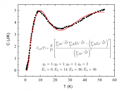
Fit Summation

This example is to fit data to a function with multiple summation series. The Nelder-Mead Simplex algorithm is used to obtain the fitting parameters in a vector form.

import numpy as np
from scipy.optimize import minimize
import originpro as op

def fitfunc(a):
    y1 = np.array(y)  
    y1 = y1.reshape(1,len(y1))
    return sum(np.square(sum(C_csk(a, x) - y1))) 
    
def C_csk(a, x):
    """
    D:DD
    """
    a = np.array(a)
    a = a.reshape(len(a),1)
    g = a[0:int(len(a)/2)]
    d = a[int(len(a)/2):]
    x1 = np.array(x)
    x1 = x1.reshape(1,len(x1))    
    m0 = g*np.exp(-d/x1)
    m1 = g*d*np.exp(-d/x1)
    m2 = g*np.square(d)*np.exp(-d/x1)
    sm = (m0.sum(axis=0)*m2.sum(axis=0) - np.square(m1.sum(axis=0)))/np.square(m0.sum(axis=0))*8.314/x1/x1
    return sm.sum(axis=0)  

def fitSummation():
    global x, y
    wks = op.find_sheet()
    x = wks.to_list(0)
    y = wks.to_list(1)
    a0 = np.array(wks.to_list(2))
    res = minimize(fitfunc, a0, method='nelder-mead', options={'xatol': 1e-8, 'disp': True})
    wks.from_list(3, res.x)

How to Execute Python Code from a Button

LabTalk script can be set up to execute from graph objects such as text labels. Script can be made to execute on events such as clicking, moving and resizing.

The examples described in previous sections use text labels set up as buttons, to execute LabTalk script. The script then executes Python code attached to the project. The following mini tutorial will show you how.

Open Code Builder from Origin (menu: View->Code Builder).
Use the menu File->New... and in the dialog select Python File, and give it the name test and click OK.
In the editor on the right side, enter the Python code:
```
print('Hello from Python!')
```
and click the Save button to save the file.
In the left panel of Code Builder, right-click on the Project node and select the context menu Add File.... Select the file test.py that you created, and click OK. The file is now attached to the project.
Go back to Origin.
Make a graph or worksheet window active.
Select the Text tool from the Tools toolbar to the left side of the Origin interface.
Click on an open space on your graph or worksheet. This will put you into text edit mode. Type Run Code in the text object and click outside the object.
Now hold down the ALT key while double-clicking on the text object that you just created. The Object Properties dialog opens to the Programming tab.
Change the Script Run After drop-down to Button Up.
In the lower text box, enter this script:
```
run -pyp test.py;
```
. This line of script tells Origin to execute the Python code contained in the file test.py which is attached to the project.
Click OK to close the dialog.
Note that the text label is now a button. Click on the button. The Script Window will open and show the output from the Python print statement.
You can now save the project and the python code file attached to the project will be saved with it.

Note that the Origin Project samples shipped with the installation have multiple buttons to Run Code, Show Code, Install Required Packages etc. You can hold down the ALT key and double-click on those buttons to view the script.

The Show Code Button

The above projects have a Show Code button that, when clicked, opens the Python code in the Code Builder IDE. IF there is only one .py file attached to the project, you can open that file in the IDE with a simple line of script: