5.8.3 Discriminant AnalysisDiscriminant-Analysis
Summary
The Iris flower data set, or Fisher's Iris dataset, is a multivariate dataset introduced by Sir Ronald Aylmer Fisher in 1936. This dataset is often used for illustrative purposes in many classification systems. The dataset consists of fifty samples from each of three species of Irises (iris setosa, iris virginica, and iris versicolor). Four characteristics, the length and width of sepal and petal, are measured in centimeters for each sample. We can use discriminant analysis to identify the species based on these four characteristics.
We will use a random sample of 120 rows of data to create a discriminant analysis model, and then use the remaining 30 rows to verify the accuracy of the model.
Minimum Origin Version Required: OriginPro 8.6 SR0
Discriminant Analysis
- Open a new project or a new workbook. Import the data file \Samples\Statistics\Fisher's Iris Data.dat
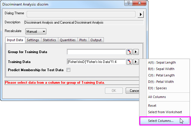
- Highlight columns A through D. and then select Statistics: Multivariate Analysis: Discriminant Analysis to open the Discriminant Analysis dialog, Input Data tab. Columns A ~ D are automatically added as Training Data.
- Click the triangle button
 next to Group for Training Data and select E(Y):Species in the context menu next to Group for Training Data and select E(Y):Species in the context menu
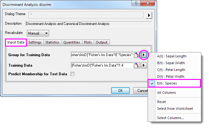
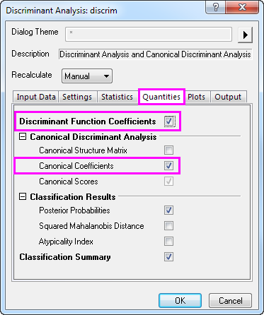
- Click the Quantities tab and select the Discriminant Function Coefficients check box. Expand the Canonical Discriminant Analysis branch and select the Canonical Coefficients check box. Accept all other default settings and click OK
Interpreting Results
Click on the Discriminant Analysis Report tab.
Canonical Discriminant Analysis
The Canonical Discriminant Analysis branch is used to create the discriminant functions for the model.
- Using the Unstandardized Canonical Coefficient table we can construct the canonical discriminant functions.
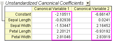   - where SL = Sepal Length, SW = Sepal Width, PL = Petal Length, PW = Petal Width
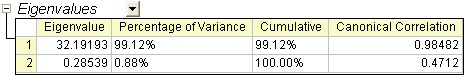
- The Eigenvalues table reveals the importance of the above canonical discriminant functions. The first function can explain 99.12% of the variance, and the second can explain the remaining 0.88%.
-
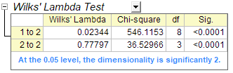
- The Wilk's Lambda Test table shows that the discriminant functions significantly explain the membership of the group. We can see that both values in the Sig column are smaller than 0.05. Both values should therefore be included in the discriminant analysis.
-
Classification
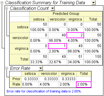
- The Classification Summary for Training Data table can be used to evaluate the discriminant model. From the table we can see that the classification in the groups setosa is 100% correct. For versicolor, only two observations are mistakenly classified as virginica, and for virginica, only one is mistakenly classified. The error rate is only 2.00%. This model is good.
- You can further switch to the Training Result1 sheet to see which observation is mistakenly classified. In the sheet we can see the post probabilities calculated from the discriminant model and which group the observation is assigned to.
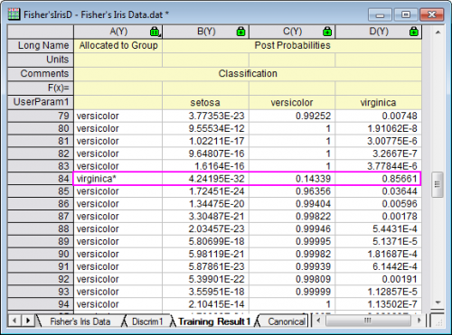
- For the 84-th observation, we can see the post probabilities(virginica) 0.85661 is the maximum value. i.e. the 84-th observation will be assigned to the group virginica (at 85.7% probability).
- But in source data, the 84-th observation is in group versicolor. So this observation is mistakenly classified by the model.
Model Validation
Model validation can be used to ensure the stability of the discriminant analysis classifiers
There are two methods to do the model validation
- Cross-validation:
- In cross-validation, each training data is treated as the test data, exclude it from training data to judge which group it should be classified as, and then verify whether the classification is correct or not.
- Subset Validation:
- Usually we will randomly divide the set of observations into subsets, the first of which is used for the estimation of discriminant model (training set) and the second is for testing the reliability of the results (test set).
Preparing Data for Analysis
We are going to sort the data in random order, and then use the first 120 rows of data as training data and the last 30 as test data.
- Go back to sheet Fisher's Iris Data
- Add a new column and fill the column with Normal Random Numbers.
- Select the newly added column. Right-click and select Sort Worksheet: Ascending from the shortcut menu.
| Notes: Origin will generate different random data each time, and different data will result in different results.
In order to get the same results as shown in this tutorial, you could open the Tutorial Data.opj under the Samples folder, browse in the Project Explorer and navigate to the Discriminant Analysis (Pro Only) subfolder, then use the data from column (F) in the Fisher's Iris Data worksheet, which is a previously generated dataset of random numbers.
|
Run Discriminant Analysis
- Select columns A through D.
- Select Statistics: Multivariate Analysis: Discriminant Analysis to open the Discriminant Analysis dialog.
- To set the first 120 rows of columns A through D as Training Data, click the triangle button next to Training Data, and then select Select Columns in the context menu.
- In the Column Browser dialog, click the ... button in the lower panel. Set data range from 1 to 120. Click OK.
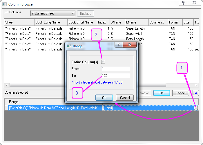
- To set first 120 rows of Col(E) as Group for Training Data, click the triangle button next to Group for Training Data and select E(Y): Species in the context menu. Then click the Group for Training Data triangle button again, select Select Columns in the context menu, and set range from 1 to 120 with column browser. Click OK.
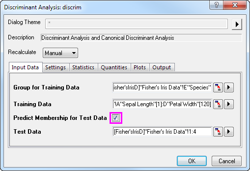
- Select Predict Membership of Test Data check box. Click the Test Data interactive button
 . The dialog will "roll up". Select columns A through D in the worksheet. Click the button in the rolled up dialog to restore the dialog. Then click the triangle button to open Column Browser by selecting Select Columns in the context menu. Click ... button in lower panel, and set range from 121 through 150. . The dialog will "roll up". Select columns A through D in the worksheet. Click the button in the rolled up dialog to restore the dialog. Then click the triangle button to open Column Browser by selecting Select Columns in the context menu. Click ... button in lower panel, and set range from 121 through 150.
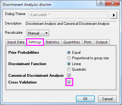
- Click the Settings tab and select the Cross Validation check box. Click OK.
Cross-validation
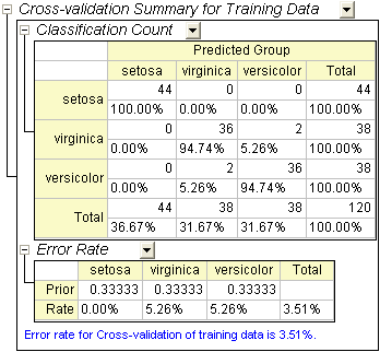
- Go to sheet Discriminant Analysis Report1. The Cross-validation Summary for Training Data table provides prediction error rate by classifying each case while leaving it out from the model calculations. However, this method is still more "optimistic" than subset validation.
Subset Validation
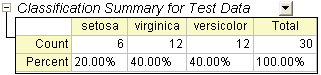
- The Classification Summary for Test Data provide information that how the test data are classified.
-
- On the worksheet Fisher's Iris Data, copy the last 30 rows (121 through 150) of Col(E): Species.
- On the worksheet Test Result, add one column, Col(E), to the worksheet. Paste the copied values in the new column.
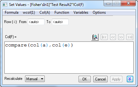
- Add a new column, Col(F) to the worksheet, right click on it and select Set Column Values in the context menu. In the opened dialog, type Compare(col(A),col(E)) in the pop-up dialog and click OK.
-
- None of 30 values is 0, it means the error rate the testing data is 0. Our discriminant model is pretty good.
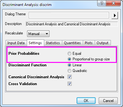
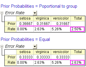
Adjusting Prior Probabilities
Discriminant analysis assumes that prior probabilities of group membership are identifiable. If group population size is unequal, prior probabilities may differ. We can use Proportional to group size for the Prior Probabilities option in this case.
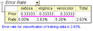
- Go to sheet Discrim2, Prior row of the Error Rate table under Classification Summary for Training Data branch indicate the prior probabilities for membership in groups. It is assumed that a case is equally likely to be one of the three groups. Adjusting the prior probabilities according to the group size can improve the overall classification rate.
- Click on the
 button and select Change Parameter from the context menu. Select Proportional to group size for Prior Probabilities radio box. Click OK button. button and select Change Parameter from the context menu. Select Proportional to group size for Prior Probabilities radio box. Click OK button.
- We can see the classification error rate is 2.50%, it is better than 2.63%, error rate with equal prior probabilities.
|