Find peaks using various search methods
This feature is updated in 8.0 SR5. For more details, please refer to Release Notes.
pkfind method:=first; // pick peaks by using the first derivative method.
Please refer to the page for additional option switches when accessing the x-function from script
| Display Name |
Variable Name |
I/O and Type |
Default Value |
Description |
|---|---|---|---|---|
| Input | iy |
Input XYRange |
|
Specify the input data. |
| Smooth Points | smooth |
Input int |
|
Savitzky-Golay smoothing can be performed to the spectrum data before the peak finding. If you want to perform the smoothing, specify the desired number of points (a positive integer) in the moving window for the Savitzky-Golay smoothing with this variable. If you do not want to perform the smoothing, set this variable to 0. |
| Direction | dir |
Input int |
|
Specify the direction of the peaks.
Option list:
|
| Method | method |
Input int |
|
Specify the method used to find the peaks.
Option list:
|
| Local Points | npts |
Input int |
|
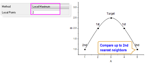
This is available only when the method variable is 0 (max). It specifies the number of points in the local area, which will be used for finding the peaks with the Local Maximum method. |
| Size Option | option |
Input int |
|
This is available only when the method variable is 1 (win). It specifies how the values for the height and width variable (see below) are interpreted.
Option list:
|
| Height | height |
Input double |
|
This is available only when the method variable is 1 (win). It specifies the height of the rectangle, which is used to find the peaks. |
| Width | width |
Input double |
|
This is available only when the method variable is 1 (win). It specifies the width of the rectangle, which is used to find the peaks. |
| Filter Peaks by | filter |
Input int |
|
Specify whether you want to limit the number of found peaks or the height of the peaks.
Option list:
|
| Threshold Height / Number of Peaks / Threshold Height(%) | value |
Input double |
|
This variable works with the filter variable above. It specifies the minimum height of the found peaks / the maximum number of the found peaks/ height percent of the found peaks |
| Maximum Half Width | hwidth |
Input double |
|
Specify the maximum range for searching the peak markers. |
| Foot Height | fheight |
Input double |
|
Specify the threshold height for searching the peak markers. |
| Center Peaks Indices | ocenter |
Output vector |
|
Output the the indices of peak centers by default. Specify where to output the indices of peak centers. |
| Left Markers Indices | oleft |
Output vector |
|
Specify whether to output the indeces of the left peak markers. |
| Right Markers Indices | oright |
Output vector |
|
Specify whether to output the indeces of the right peak markers. |
| Xs of Peak Centers | ocenter_x |
Output vector |
|
Specify whether to output the X values of the peak centers. |
| Ys of Peak Centers | ocenter_y |
Output vector |
|
Specify whether to output the Y values of the peak centers. |
| Xs of Left Markers | oleft_x |
Output vector |
|
Specify whether to output the X values of the left markers. |
| Ys of Left Markers | oleft_y |
Output vector |
|
Specify whether to output the Y values of left markers. |
| Xs of Right Markers | oright_x |
Output vector |
|
Specify whether to output the X values of the right markers. |
| Ys of Right Markers | oright_y |
Output vector |
|
Specify whether to output the Y values of the right markers. |
This X-Function can be used to find peaks (peak centers and peak markers) with various methods and output the indices of peak centers .
/*
This example shows you how to detect peaks in spectrum data.
The sample data used is in
  \Samples\Spectroscopy folder.
1. Import the sample data into a book in Origin.
2. Use the pkfind X-Function to locate the peaks.
3. Plot the original data and the found peaks.
*/
//Import spectrum data with 7 peaks
string fname$=system.path.program$ + "Samples\Spectroscopy\HiddenPeaks.dat";
newbook sheet:=0;
newsheet cols:=5 labels:="Time|Spectrum Data|Peak Center Indices|Peak Center X|Peak Center Y";
impASC;
string bkn$=%H;

//Find peak centers
pkFind iy:=col(2) method:=second ocenter:=col(3) oleft:=<none> oright:=<none> ;

//Find peak center positions by their indeces
col(4)=col(1)[col(3)];	//X positions
col(5)=col(2)[col(3)];	//Y positions
//Plot spetrum data as a black line
plotxy iy:=col(2) plot:=200;
//Plot peak centers as red scatters
plotxy iy:=[bkn$]1!(4,5) plot:=201  legend:=1 color:=2 ogl:=1!;
This X-Function provides 5 methods to find peaks. Usually, ordinary peaks can be easily found by the Local Maximum, Window Search and First Derivative methods. If your data contains hidden peaks, more sophisticated methods like Second Derivative method and Residual after First Derivative method should be used.
The peak finding is based on local extrema (maximum or minimum). The steps are as follows:
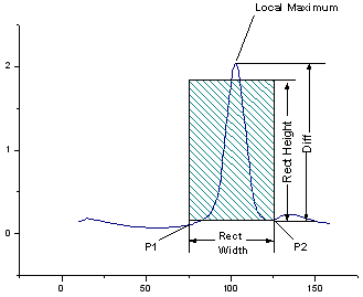
This X-Function picks the peaks with a moving rectangle, which has two sides paralleled to the X axis and the other two sides paralleled to the Y axis. The following four steps are performed so as to find whether a positive peak exists:
1.Suppose the x coordinate of the bottom-left corner of the rectangle is x1, and the x coordinate of its bottom-right corner of the rectangle is x2. We find a point P1 (x1, y1) on the input curve, whose x value is x1, and another point P2 (x2, y2) on the curve, whose x value is x2.
2.We compare y1 and y2 and take the larger of the two as y':
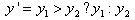
3.The local maximum of the curve (yLocalMax), which is the maximum y value on the curve between P1 and P2, is found. Then, we compute the difference between the local maximum and y' as follows:
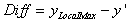
4.Compare Diff with the rectangle height. If 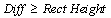 , the local maximum point will be regarded as a positive peak; otherwise, no positive peaks will be picked within this rectangle.
The procedure for finding a negative peak is similar:
1.Suppose the x coordinate of the bottom-left corner of the rectangle is x1, and the x coordinate of its bottom-right corner of the rectangle is x2. We find a point Q1 (x1, y1) on the input curve, whose x value is x1, and another point Q2 (x2, y2) on the curve, whose x value is x2.
2.We compare y1 and y2 and take the lesser of the two as y":
3.The local minimum of the curve (yLocalMin), which is the minimum y value on the curve between Q1 and Q2, is found. Then, we compute the difference between the local minimum and y" as follows:
4.Compare Diff" with the rectangle height. If 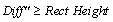 , the local minimum point will be regarded as a negative peak; otherwise, no negative peaks will be picked within this rectangle.
After these steps are completed, the rectangle will be moved 1 point toward the right and these steps are performed again, until the rectangle is out of the data range.
The basic idea of this method is as follows:
1) A positive peak center locates in a position  , where the first derivative at
  is positive while the first derivative at
  is negative;
2) A negative peak center locates in a position , where the first derivative at -1 is negative while the first derivative at +1 is positive.
is negative;
2) A negative peak center locates in a position , where the first derivative at -1 is negative while the first derivative at +1 is positive.
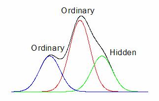
The smoothed second derivative of the data is capable of detecting local extrema in the raw data, which corresponds to peak positions of both ordinary and hidden peaks.
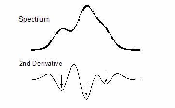
In the figure, the spectrum consists of two local maxima peaks and one hidden peaks. Its second derivative curve is shown in the lower plot, in which the hidden peak is revealed by the local minima.
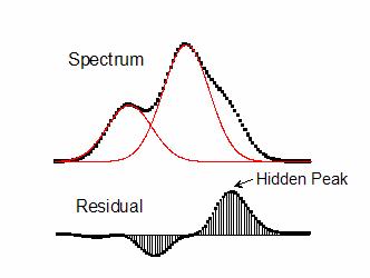
The basic ideal is as follows:
1. Use the First Derivative method to find peaks and fit the peaks individually. Then cumulate the fitting curves of every peak.
2. Calculate the residuals between the spectrum data and the cumulated fitting data.
3. The points whose corresponding residuals are greater than a threshold will be considered as hidden peaks.
Following is an example using Residual after First Derivative method to find hidden peaks. The spectrum contains two positive peaks and one hidden peak. When the cumulated data of the fitting curves of the two positive peaks are subtracted from the spectrum, the hidden peak is clearly revealed in its residual plot.
blauto, fitpeaks, pa, PaMultiY, NLfitpeaks
Keywords:spectrum, second derivative, local maximum, window, threshold