NAG Library Function Document

nag_opt_nlp_solve (e04wdc)

1

Purpose

2

Specification

3

Description

nag_opt_nlp_init(&state, ...);
nag_opt_nlp_option_set_file(ispecs, &state, ...);
nag_opt_nlp_solve(n, nclin, ncnln, ...);

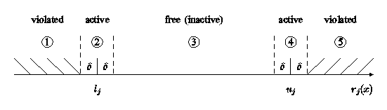
Figure 1 illustrates the feasible region for the $j$th pair of constraints $l_j\le r_j\left(x\right)\le u_j$. The quantity of $\delta$ is the $\mathbf{Feasibility\; Tolerance}$, which can be set by you (see Section 12). The constraints $l_j\le r_j\le u_j$ are considered ‘satisfied’ if $r_j$ lies in Regions 2, 3 or 4, and ‘inactive’ if $r_j$ lies in Region 3. The constraint $r_j\ge l_j$ is considered ‘active’ in Region 2, and ‘violated’ in Region 1. Similarly, $r_j\le u_j$ is active in Region 4, and violated in Region 5. For equality constraints ($l_j=u_j$), Regions 2 and 4 are the same and Region 3 is empty.

Figure 1: Illustration of the constraints $l_j\le r_j\left(x\right)\le u_j$ 

4

References

5

Arguments

1:    $\mathbf{n}$ – IntegerInput

On entry: $n$, the number of variables.

Constraint: $\mathbf{n}>0$.

2:    $\mathbf{nclin}$ – IntegerInput

On entry: $n_L$, the number of general linear constraints.

Constraint: $\mathbf{nclin}\ge 0$.

3:    $\mathbf{ncnln}$ – IntegerInput

On entry: $n_N$, the number of nonlinear constraints.

Constraint: $\mathbf{ncnln}\ge 0$.

4:    $\mathbf{tda}$ – IntegerInput

On entry: the stride separating matrix column elements in the array a.

Constraints:

• if $\mathbf{nclin}>0$, $\mathbf{tda}\ge \mathbf{n}$;
• otherwise $\mathbf{tda}\ge 1$.

5:    $\mathbf{tdcj}$ – IntegerInput

On entry: the stride separating matrix column elements in the array cjac.

Constraints:

• if $\mathbf{ncnln}>0$, $\mathbf{tdcj}\ge \mathbf{n}$;
• otherwise $\mathbf{tdcj}\ge 1$.

6:    $\mathbf{tdh}$ – IntegerInput

On entry: the stride separating matrix column elements in the array h.

Constraint: $\mathbf{tdh}\ge \mathbf{n}$ unless the optional parameter $\mathbf{Hessian\; Limited\; Memory}$ is in effect. If $\mathbf{Hessian\; Limited\; Memory}$ is in effect, array h is not referenced

7:    $\mathbf{a}\left[\mathit{dim}\right]$ – const doubleInput

Note: the dimension, dim, of the array a must be at least $\max \left(1,\mathbf{nclin}\times \mathbf{tda}\right)$.

The $\left(i,j\right)$th element of the matrix $A$ is stored in $\mathbf{a}\left[\left(i-1\right)\times \mathbf{tda}+j-1\right]$.

On entry: the $\mathit{i}$th row of a contains the $\mathit{i}$th row of the matrix $A_L$ of general linear constraints in (1). That is, the $\mathit{i}$th row contains the coefficients of the $\mathit{i}$th general linear constraint, for $\mathit{i}=1,2,\dots ,\mathbf{nclin}$.

If $\mathbf{nclin}=0$, the array a is not referenced.

8:    $\mathbf{bl}\left[\mathbf{n}+\mathbf{nclin}+\mathbf{ncnln}\right]$ – const doubleInput

9:    $\mathbf{bu}\left[\mathbf{n}+\mathbf{nclin}+\mathbf{ncnln}\right]$ – const doubleInput

On entry: bl must contain the lower bounds and bu the upper bounds for all the constraints, in the following order. The first $n$ elements of each array must contain the bounds on the variables, the next $n_L$ elements the bounds for the general linear constraints (if any) and the next $n_N$ elements the bounds for the general nonlinear constraints (if any). To specify a nonexistent lower bound (i.e., $l_j=-\infty$), set $\mathbf{bl}\left[j-1\right]\le -\mathit{bigbnd}$, and to specify a nonexistent upper bound (i.e., $u_j=+\infty$), set $\mathbf{bu}\left[j-1\right]\ge \mathit{bigbnd}$; where $\mathit{bigbnd}$ is the optional parameter $\mathbf{Infinite\; Bound\; Size}$. To specify the $j$th constraint as an equality, set $\mathbf{bl}\left[j-1\right]=\mathbf{bu}\left[j-1\right]=\beta$, say, where $\left|\beta \right|<\mathit{bigbnd}$.

Constraints:

• $\mathbf{bl}\left[\mathit{j}-1\right]\le \mathbf{bu}\left[\mathit{j}-1\right]$, for $\mathit{j}=1,2,\dots ,\mathbf{n}+\mathbf{nclin}+\mathbf{ncnln}$;
• if $\mathbf{bl}\left[j-1\right]=\mathbf{bu}\left[j-1\right]=\beta$, $\left|\beta \right|<\mathit{bigbnd}$.

10:  $\mathbf{confun}$ – function, supplied by the userExternal Function

confun must calculate the vector $c\left(x\right)$ of nonlinear constraint functions and (optionally) its Jacobian, $\frac{\partial c}{\partial x}$, for a specified $n$-vector $x$. If there are no nonlinear constraints (i.e., $\mathbf{ncnln}=0$), nag_opt_nlp_solve (e04wdc) will never call confun, so it may be specified as NULLFN. If there are nonlinear constraints, the first call to confun will occur before the first call to objfun.

If all constraint gradients (Jacobian elements) are known (i.e., $\mathbf{Derivative\; Level}=2$ or $3$), any constant elements may be assigned to cjac once only at the start of the optimization. An element of cjac that is not subsequently assigned in confun will retain its initial value throughout. Constant elements may be loaded in cjac during the first call to confun (signalled by the value of $\mathbf{nstate}=1$). The ability to preload constants is useful when many Jacobian elements are identically zero, in which case cjac may be initialized to zero and nonzero elements may be reset by confun.

It must be emphasized that, if $\mathbf{Derivative\; Level}<2$, unassigned elements of cjac are not treated as constant; they are estimated by finite differences, at nontrivial expense.

The specification of confun is:

void  confun (Integer *mode, Integer ncnln, Integer n, Integer tdcj, const Integer needc[], const double x[], double ccon[], double cjac[], Integer nstate, Nag_Comm *comm)

1:    $\mathbf{mode}$ – Integer *Input/Output

On entry: is set by nag_opt_nlp_solve (e04wdc) to indicate which values must be assigned during each call of confun. Only the following values need be assigned, for each value of $i$ such that $\mathbf{needc}\left[i-1\right]>0$:

$\mathbf{mode}=0$

The components of ccon corresponding to positive values in needc must be set. Other components and the array cjac are ignored.

$\mathbf{mode}=1$

The known components of the rows of cjac corresponding to positive values in needc must be set. Other rows of cjac and the array ccon will be ignored.

$\mathbf{mode}=2$

Only the elements of ccon corresponding to positive values of needc need to be set (and similarly for the known components of the rows of cjac).

On exit: may be used to indicate that you are unable or unwilling to evaluate the constraint functions at the current $x$.

During the linesearch, the constraint functions are evaluated at points of the form $x=x_k+\alpha p_k$ after they have already been evaluated satisfactorily at $x_k$. At any such $\alpha$, if you set $\mathbf{mode}=-1$, nag_opt_nlp_solve (e04wdc) will evaluate the functions at some point closer to $x_k$ (where they are more likely to be defined).

If for some reason you wish to terminate the current problem, set $\mathbf{mode}<-1$.

2:    $\mathbf{ncnln}$ – IntegerInput

On entry: $n_N$, the number of nonlinear constraints.

3:    $\mathbf{n}$ – IntegerInput

On entry: $n$, the number of variables.

4:    $\mathbf{tdcj}$ – IntegerInput

On entry: the stride used in the array cjac.

5:    $\mathbf{needc}\left[\mathbf{ncnln}\right]$ – const IntegerInput

On entry: the indices of the elements of ccon and/or cjac that must be evaluated by confun. If $\mathbf{needc}\left[i-1\right]>0$, the $i$th element of ccon and/or the available elements of the $i$th row of cjac (see argument mode) must be evaluated at $x$.

6:    $\mathbf{x}\left[\mathbf{n}\right]$ – const doubleInput

On entry: $x$, the vector of variables at which the constraint functions and/or the available elements of the constraint Jacobian are to be evaluated.

7:    $\mathbf{ccon}\left[\max \left(1,\mathbf{ncnln}\right)\right]$ – doubleOutput

On exit: if $\mathbf{needc}\left[i-1\right]>0$ and $\mathbf{mode}=0$ or $2$, $\mathbf{ccon}\left[i-1\right]$ must contain the value of the $i$th constraint at $x$. The remaining elements of ccon, corresponding to the non-positive elements of needc, are ignored.

8:    $\mathbf{cjac}\left[\mathbf{ncnln}\times \mathbf{tdcj}\right]$ – doubleInput/Output

On entry: the elements of cjac are set to special values that enable nag_opt_nlp_solve (e04wdc) to detect whether they are reset by confun.

On exit: if $\mathbf{needc}\left[i-1\right]>0$ and $\mathbf{mode}=1$ or $2$, the $i$th row of cjac must contain the available elements of the vector $\nabla c_i$ given by

$$\nabla c_i={\left(\frac{\partial c_i}{\partial x_1},\frac{\partial c_i}{\partial x_2},\dots ,\frac{\partial c_i}{\partial x_n}\right)}^{\mathrm{T}}\text{,}$$

where $\frac{\partial c_i}{\partial x_j}$ is the partial derivative of the $i$th constraint with respect to the $j$th variable, evaluated at the point $x$. See also the argument nstate. The remaining rows of cjac, corresponding to non-positive elements of needc, are ignored.

If all elements of the constraint Jacobian are known (i.e., $\mathbf{Derivative\; Level}=2$ or $3$), any constant elements may be assigned to cjac one time only at the start of the optimization. An element of cjac that is not subsequently assigned in confun will retain its initial value throughout. Constant elements may be loaded into cjac during the first call to confun (signalled by the value $\mathbf{nstate}=1$). The ability to preload constants is useful when many Jacobian elements are identically zero, in which case cjac may be initialized to zero and nonzero elements may be reset by confun.

Note that constant nonzero elements do affect the values of the constraints. Thus, if $\mathbf{cjac}\left[\left(i-1\right)\times \mathbf{tdcj}+j-1\right]$ is set to a constant value, it need not be reset in subsequent calls to confun, but the value $\mathbf{cjac}\left[\left(i-1\right)\times \mathbf{tdcj}+j-1\right]\times \mathbf{x}\left[j-1\right]$ must nonetheless be added to $\mathbf{ccon}\left[i-1\right]$. For example, if $\mathbf{cjac}\left[0\right]=2$ and $\mathbf{cjac}\left[1\right]=-5$ then the term $2\times \mathbf{x}\left[0\right]-5\times \mathbf{x}\left[1\right]$ must be included in the definition of $\mathbf{ccon}\left[0\right]$.

It must be emphasized that, if $\mathbf{Derivative\; Level}=0$ or $1$, unassigned elements of cjac are not treated as constant; they are estimated by finite differences, at nontrivial expense. If you do not supply a value for the optional parameter $\mathbf{Difference\; Interval}$, an interval for each element of $x$ is computed automatically at the start of the optimization. The automatic procedure can usually identify constant elements of cjac, which are then computed once only by finite differences.

9:    $\mathbf{nstate}$ – IntegerInput

On entry: if $\mathbf{nstate}=1$ then nag_opt_nlp_solve (e04wdc) is calling confun for the first time. This argument setting allows you to save computation time if certain data must be read or calculated only once.

10:  $\mathbf{comm}$ – Nag_Comm *

Pointer to structure of type Nag_Comm; the following members are relevant to confun.

user – double *

iuser – Integer *

p – Pointer 

The type Pointer will be void *. Before calling nag_opt_nlp_solve (e04wdc) you may allocate memory and initialize these pointers with various quantities for use by confun when called from nag_opt_nlp_solve (e04wdc) (see Section 3.3.1.1 in How to Use the NAG Library and its Documentation).

Note: confun should not return floating-point NaN (Not a Number) or infinity values, since these are not handled by nag_opt_nlp_solve (e04wdc). If your code inadvertently does return any NaNs or infinities, nag_opt_nlp_solve (e04wdc) is likely to produce unexpected results.

confun should be tested separately before being used in conjunction with nag_opt_nlp_solve (e04wdc). See also the description of the optional parameter $\mathbf{Verify\; Level}$.

11:  $\mathbf{objfun}$ – function, supplied by the userExternal Function

objfun must calculate the objective function $F\left(x\right)$ and (optionally) its gradient $g\left(x\right)=\frac{\partial F}{\partial x}$ for a specified $n$-vector $x$.

The specification of objfun is:

void  objfun (Integer *mode, Integer n, const double x[], double *objf, double grad[], Integer nstate, Nag_Comm *comm)

1:    $\mathbf{mode}$ – Integer *Input/Output

On entry: is set by nag_opt_nlp_solve (e04wdc) to indicate which values must be assigned during each call of objfun. Only the following values need be assigned:

$\mathbf{mode}=0$

objf.

$\mathbf{mode}=1$

All available elements of grad.

$\mathbf{mode}=2$

objf and all available elements of grad.

On exit: may be used to indicate that you are unable or unwilling to evaluate the objective function at the current $x$.

During the linesearch, the function is evaluated at points of the form $x=x_k+\alpha p_k$ after they have already been evaluated satisfactorily at $x_k$. For any such $x$, if you set $\mathbf{mode}=-1$, nag_opt_nlp_solve (e04wdc) will reduce $\alpha$ and evaluate the functions again (closer to $x_k$, where they are more likely to be defined).

If for some reason you wish to terminate the current problem, set $\mathbf{mode}<-1$.

2:    $\mathbf{n}$ – IntegerInput

On entry: $n$, the number of variables.

3:    $\mathbf{x}\left[\mathbf{n}\right]$ – const doubleInput

On entry: $x$, the vector of variables at which the objective function and/or all available elements of its gradient are to be evaluated.

4:    $\mathbf{objf}$ – double *Output

On exit: if $\mathbf{mode}=0$ or $2$, objf must be set to the value of the objective function at $x$.

5:    $\mathbf{grad}\left[\mathbf{n}\right]$ – doubleInput/Output

On entry: the elements of grad are set to special values.

On exit: if $\mathbf{mode}=1$ or $2$, grad must return the available elements of the gradient evaluated at $x$, i.e., $\mathbf{grad}\left[i-1\right]$ contains the partial derivative $\frac{\partial F}{\partial x_i}$.

6:    $\mathbf{nstate}$ – IntegerInput

On entry: if $\mathbf{nstate}=1$ then nag_opt_nlp_solve (e04wdc) is calling objfun for the first time. This argument setting allows you to save computation time if certain data must be read or calculated only once.

7:    $\mathbf{comm}$ – Nag_Comm *

Pointer to structure of type Nag_Comm; the following members are relevant to objfun.

user – double *

iuser – Integer *

p – Pointer 

The type Pointer will be void *. Before calling nag_opt_nlp_solve (e04wdc) you may allocate memory and initialize these pointers with various quantities for use by objfun when called from nag_opt_nlp_solve (e04wdc) (see Section 3.3.1.1 in How to Use the NAG Library and its Documentation).

Note: objfun should not return floating-point NaN (Not a Number) or infinity values, since these are not handled by nag_opt_nlp_solve (e04wdc). If your code inadvertently does return any NaNs or infinities, nag_opt_nlp_solve (e04wdc) is likely to produce unexpected results.

objfun should be tested separately before being used in conjunction with nag_opt_nlp_solve (e04wdc). See also the description of the optional parameter $\mathbf{Verify\; Level}$.

12:  $\mathbf{majits}$ – Integer *Output

On exit: the number of major iterations performed.

13:  $\mathbf{istate}\left[\mathbf{n}+\mathbf{nclin}+\mathbf{ncnln}\right]$ – IntegerInput/Output

On entry: is an integer array that need not be initialized if nag_opt_nlp_solve (e04wdc) is called with the $\mathbf{Cold\; Start}$ option (the default).

If optional parameter $\mathbf{Warm\; Start}$ has been chosen, every element of istate must be set. If nag_opt_nlp_solve (e04wdc) has just been called on a problem with the same dimensions, istate already contains valid values. Otherwise, $\mathbf{istate}\left[j-1\right]$ should indicate whether either of the constraints $r_j\left(x\right)\ge l_j$ or $r_j\left(x\right)\le u_j$ is expected to be active at a solution of (1).

The ordering of istate is the same as for bl, bu and $r\left(x\right)$, i.e., the first n components of istate refer to the upper and lower bounds on the variables, the next nclin refer to the bounds on $A_{L}x$, and the last ncnln refer to the bounds on $c\left(x\right)$. Possible values of $\mathbf{istate}\left[i-1\right]$ follow:

$0$	Neither $r_j\left(x\right)\ge l_j$ nor $r_j\left(x\right)\le u_j$ is expected to be active.
$1$	$r_j\left(x\right)\ge l_j$ is expected to be active.
$2$	$r_j\left(x\right)\le u_j$ is expected to be active.
$3$	This may be used if $l_j=u_j$. Normally an equality constraint $r_j\left(x\right)=l_j=u_j$ is active at a solution.

The values $1$, $2$ or $3$ all have the same effect when $\mathbf{bl}\left[j-1\right]=\mathbf{bu}\left[j-1\right]$. If necessary, nag_opt_nlp_solve (e04wdc) will override your specification of istate, so that a poor choice will not cause the algorithm to fail.

On exit: describes the status of the constraints $l\le r\left(x\right)\le u$. For the $j$th lower or upper bound, $j=1,2,\dots ,\mathbf{n}+\mathbf{nclin}+\mathbf{ncnln}$, the possible values of $\mathbf{istate}\left[j-1\right]$ are as follows (see Figure 1). $\delta$ is the appropriate feasibility tolerance.

$-2$	(Region 1) The lower bound is violated by more than $\delta$.
$-1$	(Region 5) The upper bound is violated by more than $\delta$.
$\phantom{-}0$	(Region 3) Both bounds are satisfied by more than $\delta$.
$\phantom{-}1$	(Region 2) The lower bound is active (to within $\delta$).
$\phantom{-}2$	(Region 4) The upper bound is active (to within $\delta$).
$\phantom{-}3$	($\text{Region 2}=\text{Region 4}$) The bounds are equal and the equality constraint is satisfied (to within $\delta$).

These values of istate are labelled in the printed solution according to Table 1.

Region	$1$	$2$	$3$	$4$	$5$	$2\equiv 4$
$\mathbf{istate}\left[j-1\right]$	$-2$	$1$	$0$	$2$	$-1$	$3$
Printed solution	--	LL	FR	UL	++	EQ

Table 1
Labels used in the printed solution for the regions in Figure 1

14:  $\mathbf{ccon}\left[\max \left(1,\mathbf{ncnln}\right)\right]$ – doubleInput/Output

On entry: ccon need not be initialized if the (default) optional parameter $\mathbf{Cold\; Start}$ is used.

For a $\mathbf{Warm\; Start}$, and if $\mathbf{ncnln}>0$, ccon contains values of the nonlinear constraint functions $c_{\mathit{i}}$, for $\mathit{i}=1,2,\dots ,\mathbf{ncnln}$, calculated in a previous call to nag_opt_nlp_solve (e04wdc).

On exit: if $\mathbf{ncnln}>0$, $\mathbf{ccon}\left[\mathit{i}-1\right]$ contains the value of the $\mathit{i}$th nonlinear constraint function $c_{\mathit{i}}$ at the final iterate, for $\mathit{i}=1,2,\dots ,\mathbf{ncnln}$.

If $\mathbf{ncnln}=0$, the array ccon is not referenced.

15:  $\mathbf{cjac}\left[\mathit{dim}\right]$ – doubleInput/Output

Note: the dimension, dim, of the array cjac must be at least $\max \left(1,\mathbf{ncnln}\times \mathbf{tdcj}\right)$.

On entry: in general, cjac need not be initialized before the call to nag_opt_nlp_solve (e04wdc). However, if $\mathbf{Derivative\; Level}=2$ or $3$, any constant elements of cjac may be initialized. Such elements need not be reassigned on subsequent calls to confun.

On exit: if $\mathbf{ncnln}>0$, cjac contains the Jacobian matrix of the nonlinear constraint functions at the final iterate, i.e., $\mathbf{cjac}\left[\left(\mathit{i}-1\right)\times \mathbf{tdcj}+\mathit{j}-1\right]$ contains the partial derivative of the $\mathit{i}$th constraint function with respect to the $\mathit{j}$th variable, for $\mathit{i}=1,2,\dots ,\mathbf{ncnln}$ and $\mathit{j}=1,2,\dots ,\mathbf{n}$. (See the discussion of argument cjac under confun.)

If $\mathbf{ncnln}=0$, the array cjac is not referenced.

16:  $\mathbf{clamda}\left[\mathbf{n}+\mathbf{nclin}+\mathbf{ncnln}\right]$ – doubleInput/Output

On entry: need not be set if the (default) optional parameter $\mathbf{Cold\; Start}$ is used.

If the optional parameter $\mathbf{Warm\; Start}$ has been chosen, $\mathbf{clamda}\left[\mathit{j}-1\right]$ must contain a multiplier estimate for each nonlinear constraint, with a sign that matches the status of the constraint specified by the istate array, for $\mathit{j}=\mathbf{n}+\mathbf{nclin}+1,\dots ,\mathbf{n}+\mathbf{nclin}+\mathbf{ncnln}$. The remaining elements need not be set. If the $j$th constraint is defined as ‘inactive’ by the initial value of the istate array (i.e., $\mathbf{istate}\left[j-1\right]=0$), $\mathbf{clamda}\left[j-1\right]$ should be zero; if the $j$th constraint is an inequality active at its lower bound (i.e., $\mathbf{istate}\left[j-1\right]=1$), $\mathbf{clamda}\left[j-1\right]$ should be non-negative; if the $j$th constraint is an inequality active at its upper bound (i.e., $\mathbf{istate}\left[j-1\right]=2$), $\mathbf{clamda}\left[j-1\right]$ should be non-positive. If necessary, the function will modify clamda to match these rules.

On exit: the values of the QP multipliers from the last QP subproblem. $\mathbf{clamda}\left[j-1\right]$ should be non-negative if $\mathbf{istate}\left[j-1\right]=1$ and non-positive if $\mathbf{istate}\left[j-1\right]=2$.

17:  $\mathbf{objf}$ – double *Output

On exit: the value of the objective function at the final iterate.

18:  $\mathbf{grad}\left[\mathbf{n}\right]$ – doubleOutput

On exit: the gradient of the objective function (or its finite difference approximation) at the final iterate.

19:  $\mathbf{h}\left[\mathit{dim}\right]$ – doubleInput/Output

Note: the dimension, dim, of the array h must be at least $\mathbf{n}\times \mathbf{tdh}$.

On entry: h need not be initialized if the (default) optional parameter $\mathbf{Cold\; Start}$ is used, and will be set to the identity.

If the optional parameter $\mathbf{Warm\; Start}$ has been chosen, h provides the initial approximation of the Hessian of the Lagrangian, i.e., $\mathbf{h}\left[\left(i-1\right)\times \mathbf{tdh}+j-1\right]\approx \frac{{\partial }^2\mathcal{L}\left(x,\lambda \right)}{\partial x_i\partial x_j}$, where $\mathcal{L}\left(x,\lambda \right)=F\left(x\right)-{c\left(x\right)}^{\mathrm{T}}\lambda$ and $\lambda$ is an estimate of the Lagrange multipliers. h must be a positive definite matrix.

On exit: contains the Hessian of the Lagrangian at the final estimate $x$.

20:  $\mathbf{x}\left[\mathbf{n}\right]$ – doubleInput/Output

On entry: an initial estimate of the solution.

On exit: the final estimate of the solution.

21:  $\mathbf{state}$ – Nag_E04State *Communication Structure

state contains internal information required for functions in this suite. It must not be modified in any way.

22:  $\mathbf{comm}$ – Nag_Comm *

The NAG communication argument (see Section 3.3.1.1 in How to Use the NAG Library and its Documentation).

23:  $\mathbf{fail}$ – NagError *Input/Output

The NAG error argument (see Section 3.7 in How to Use the NAG Library and its Documentation).

nag_opt_nlp_solve (e04wdc) returns with $\mathbf{fail}\mathbf{.}\mathbf{code}=$ NE_NOERROR if the iterates have converged to a point $x$ that satisfies the first-order Kuhn–Tucker (see Section 13.2) conditions to the accuracy requested by the $\mathbf{Major\; Optimality\; Tolerance}$, i.e., the projected gradient and active constraint residuals are negligible at $x$.

You should check whether the following four conditions are satisfied:

(i)	the final value of rgNorm (see Section 13.2) is significantly less than that at the starting point;
(ii)	during the final major iterations, the values of Step and Minors (see Section 13.1) are both one;
(iii)	the last few values of both rgNorm and SumInf (see Section 13.2) become small at a fast linear rate; and
(iv)	condHz (see Section 13.1) is small.

If all these conditions hold, $x$ is almost certainly a local minimum of (1).

One caution about ‘Optimal solutions’. Some of the variables or slacks may lie outside their bounds more than desired, especially if scaling was requested. Max Primal infeas in the Print file refers to the largest bound infeasibility and which variable is involved. If it is too large, consider restarting with a smaller $\mathbf{Minor\; Feasibility\; Tolerance}$ (say $10$ times smaller) and perhaps $\mathbf{Scale\; Option}=0$.

Similarly, Max Dual infeas in the Print file indicates which variable is most likely to be at a nonoptimal value. Broadly speaking, if

$$\mathtt{Max\; Dual\; infeas}/\mathtt{Max\; pi}={10}^{-d}\text{,}$$

then the objective function would probably change in the $d$th significant digit if optimization could be continued. If $d$ seems too large, consider restarting with a smaller $\mathbf{Major\; Optimality\; Tolerance}$.

Finally, Nonlinear constraint violn in the Print file shows the maximum infeasibility for nonlinear rows. If it seems too large, consider restarting with a smaller $\mathbf{Major\; Feasibility\; Tolerance}$.

6

Error Indicators and Warnings

NE_ALLOC_FAIL

Dynamic memory allocation failed.
See Section 2.3.1.2 in How to Use the NAG Library and its Documentation for further information.

Internal error: memory allocation failed when attempting to allocate workspace sizes $〈\mathit{\text{value}}〉$ and $〈\mathit{\text{value}}〉$. Please contact NAG.

NE_ALLOC_INSUFFICIENT

Internal memory allocation was insufficient. Please contact NAG.

NE_BAD_PARAM

Basis file dimensions do not match this problem.

On entry, argument $〈\mathit{\text{value}}〉$ had an illegal value.

NE_BASIS_FAILURE

An error has occurred in the basis package, perhaps indicating incorrect setup of arrays. Set the optional parameter $\mathbf{Print\; File}$ and examine the output carefully for further information.

NE_DERIV_ERRORS

User-supplied function computes incorrect constraint derivatives.

User-supplied function computes incorrect objective derivatives.

If the message refers to the derivatives of the objective function, then a check has been made on some individual elements of the objective gradient array at the first point that satisfies the linear constraints. At least one component $\mathbf{grad}j-1$ is being set to a value that disagrees markedly with its associated forward-difference estimate $\frac{\partial F}{\partial x_j}$. (The relative difference between the computed and estimated values is $1.0$ or more.) This exit is a safeguard, since nag_opt_nlp_solve (e04wdc) will usually fail to make progress when the computed gradients are seriously inaccurate. In the process it may expend considerable effort before terminating with $\mathbf{fail}\mathbf{.}\mathbf{code}=$ NE_NUM_DIFFICULTIES.

Check the function and gradient computation very carefully in objfun. A simple omission could explain everything. If $F$ or a component $\frac{\partial F}{\partial x_j}$ is very large, then give serious thought to scaling the function or the nonlinear variables.

If you feel certain that the computed $\mathbf{grad}\left[j-1\right]$ is correct (and that the forward-difference estimate is therefore wrong), you can specify $\mathbf{Verify\; Level}=0$ to prevent individual elements from being checked. However, the optimization procedure may have difficulty.

If the message refers to derivatives of the constraints, then at least one of the computed constraint derivatives is significantly different from an estimate obtained by forward-differencing the vector $c\left(x\right)$. Follow the advice given above, trying to ensure that the arrays ccon and cjac are being set correctly in confun.

NE_E04WCC_NOT_INIT

The initialization function nag_opt_nlp_init (e04wcc) has not been called.

NE_INT

On entry, $\mathbf{n}=〈\mathit{\text{value}}〉$.
Constraint: $\mathbf{n}>0$.

On entry, $\mathbf{nclin}=〈\mathit{\text{value}}〉$.
Constraint: $\mathbf{nclin}\ge 0$.

On entry, $\mathbf{ncnln}=〈\mathit{\text{value}}〉$.
Constraint: $\mathbf{ncnln}\ge 0$.

On entry, $\mathbf{tda}=〈\mathit{\text{value}}〉$.
Constraint: $\mathbf{tda}>0$.

On entry, $\mathbf{tdcj}=〈\mathit{\text{value}}〉$.
Constraint: $\mathbf{tdcj}>0$.

On entry, $\mathbf{tdh}=〈\mathit{\text{value}}〉$.
Constraint: $\mathbf{tdh}>0$.

NE_INT_2

On entry, $\mathbf{nclin}=〈\mathit{\text{value}}〉$ and $\mathbf{n}=〈\mathit{\text{value}}〉$.
Constraint: $\mathbf{n}>0$.

On entry, $\mathbf{ncnln}=〈\mathit{\text{value}}〉$ and $\mathbf{n}=〈\mathit{\text{value}}〉$.
Constraint: $\mathbf{n}>0$.

On entry, $\mathbf{tda}=〈\mathit{\text{value}}〉$ and $\mathbf{nclin}=〈\mathit{\text{value}}〉$.
Constraint: $\mathbf{tda}\ge \mathbf{nclin}$.

On entry, $\mathbf{tdcj}=〈\mathit{\text{value}}〉$ and $\mathbf{ncnln}=〈\mathit{\text{value}}〉$.
Constraint: $\mathbf{tdcj}\ge \mathbf{ncnln}$.

On entry, $\mathbf{tdh}=〈\mathit{\text{value}}〉$ and $\mathbf{n}=〈\mathit{\text{value}}〉$.
Constraint: $\mathbf{tdh}\ge \mathbf{n}$.

NE_INT_3

On entry, $\mathbf{tda}=〈\mathit{\text{value}}〉$, $\mathbf{nclin}=〈\mathit{\text{value}}〉$ and $\mathbf{n}=〈\mathit{\text{value}}〉$.
Constraint: if $\mathbf{nclin}>0$, $\mathbf{tda}\ge \mathbf{n}$;
otherwise $\mathbf{tda}\ge 1$.

On entry, $\mathbf{tdcj}=〈\mathit{\text{value}}〉$, $\mathbf{ncnln}=〈\mathit{\text{value}}〉$ and $\mathbf{n}=〈\mathit{\text{value}}〉$.
Constraint: if $\mathbf{ncnln}>0$, $\mathbf{tdcj}\ge \mathbf{n}$;
otherwise $\mathbf{tdcj}\ge 1$.

NE_INTERNAL_ERROR

An internal error has occurred in this function. Check the function call and any array sizes. If the call is correct then please contact NAG for assistance.
See Section 2.7.6 in How to Use the NAG Library and its Documentation for further information.

An unexpected error has occurred. Set the optional parameter $\mathbf{Print\; File}$ and examine the output carefully for further information.

NE_NO_LICENCE

Your licence key may have expired or may not have been installed correctly.
See Section 2.7.5 in How to Use the NAG Library and its Documentation for further information.

NE_NOT_REQUIRED_ACC

The requested accuracy could not be achieved.

A feasible solution has been found, but the requested accuracy in the dual infeasibilities could not be achieved. An abnormal termination has occurred, but nag_opt_nlp_solve (e04wdc) is within ${10}^{-2}$ of satisfying the $\mathbf{Major\; Optimality\; Tolerance}$. Check that the $\mathbf{Major\; Optimality\; Tolerance}$ is not too small.

NE_NUM_DIFFICULTIES

Numerical difficulties have been encountered and no further progress can be made.

Numerical difficulties have been encountered and no further progress can be made.

Several circumstances could lead to this exit.

1.	The user-supplied functions objfun or confun could be returning accurate function values but inaccurate gradients (or vice versa). This is the most likely cause. Study the comments given for $\mathbf{fail}\mathbf{.}\mathbf{code}=$ NE_DERIV_ERRORS, and do your best to ensure that the coding is correct.
2.	The function and gradient values could be consistent, but their precision could be too low. For example, accidental use of a real data type when double precision was intended would lead to a relative function precision of about ${10}^{-6}$ instead of something like ${10}^{-15}$. The default $\mathbf{Major\; Optimality\; Tolerance}$ of $2\times {10}^{-6}$ would need to be raised to about ${10}^{-3}$ for optimality to be declared (at a rather suboptimal point). Of course, it is better to revise the function coding to obtain as much precision as economically possible.
3.	If function values are obtained from an expensive iterative process, they may be accurate to rather few significant figures, and gradients will probably not be available. One should specify $\mathbf{Function\; Precision}$ $t$ $\mathbf{Major\; Optimality\; Tolerance}$ $\sqrt{t}$ but even then, if $t$ is as large as ${10}^{-5}$ or ${10}^{-6}$ (only $5$ or $6$ significant figures), the same exit condition may occur. At present the only remedy is to increase the accuracy of the function calculation.
4.	An $LU$ factorization of the basis has just been obtained and used to recompute the basic variables $x_B$, given the present values of the superbasic and nonbasic variables. A step of ‘iterative refinement’ has also been applied to increase the accuracy of $x_B$. However, a row check has revealed that the resulting solution does not satisfy the current constraints $Ax-s=0$ sufficiently well. This probably means that the current basis is very ill-conditioned. If there are some linear constraints and variables, try $\mathbf{Scale\; Option}=1$ if scaling has not yet been used. For certain highly structured basis matrices (notably those with band structure), a systematic growth may occur in the factor $U$. Consult the description of Umax and Growth in Section 13.4 and set the $\mathbf{LU\; Factor\; Tolerance}$ to $2.0$ (or possibly even smaller, but not less than $1.0$).
5.	The first factorization attempt will have found the basis to be structurally or numerically singular. (Some diagonals of the triangular matrix $U$ were respectively zero or smaller than a certain tolerance.) The associated variables are replaced by slacks and the modified basis is refactorized, but singularity persists. This must mean that the problem is badly scaled, or the $\mathbf{LU\; Factor\; Tolerance}$ is too much larger than $1.0$. This is highly unlikely to occur.

NE_REAL_2

On entry, bounds bl and bu for $〈\mathit{\text{value}}〉$ are equal and infinite. $\mathbf{bl}=\mathbf{bu}=〈\mathit{\text{value}}〉$ and $\mathit{bigbnd}=〈\mathit{\text{value}}〉$.

On entry, bounds for $〈\mathit{\text{value}}〉$ are inconsistent. $\mathbf{bl}=〈\mathit{\text{value}}〉$ and $\mathbf{bu}=〈\mathit{\text{value}}〉$.

NE_UNBOUNDED

The problem appears to be unbounded. The constraint violation limit has been reached.

The problem appears to be unbounded. The objective function is unbounded.

The problem appears to be unbounded (or badly scaled).

For linear problems, unboundedness is detected by the simplex method when a nonbasic variable can be increased or decreased by an arbitrary amount without causing a basic variable to violate a bound. Consider adding an upper or lower bound to the variable. Also, examine the constraints that have nonzeros in the associated column, to see if they have been formulated as intended.

Very rarely, the scaling of the problem could be so poor that numerical error will give an erroneous indication of unboundedness. Consider using the optional parameter $\mathbf{Scale\; Option}$.

For nonlinear problems, nag_opt_nlp_solve (e04wdc) monitors both the size of the current objective function and the size of the change in the variables at each step. If either of these is very large (as judged by the ‘Unbounded’ parameters (see Section 12)), the problem is terminated and declared unbounded. To avoid large function values, it may be necessary to impose bounds on some of the variables in order to keep them away from singularities in the nonlinear functions.

The message may indicate an abnormal termination while enforcing the limit on the constraint violations. This exit implies that the objective is not bounded below in the feasible region defined by expanding the bounds by the value of the $\mathbf{Violation\; Limit}$.

NE_USER_STOP

User-supplied constraint function requested termination.

User-supplied objective function requested termination.

You have indicated the wish to terminate solution of the current problem by setting mode to a value $<-1$ on exit from objfun or confun.

NE_USRFUN_UNDEFINED

Unable to proceed into undefined region of user-supplied function.

User-supplied function is undefined at the first feasible point.

User-supplied function is undefined at the initial point.

You have indicated that the problem functions are undefined by assigning the value $\mathbf{mode}=-1$ on exit from objfun or confun. nag_opt_nlp_solve (e04wdc) attempts to evaluate the problem functions closer to a point at which the functions are already known to be defined. This exit occurs if nag_opt_nlp_solve (e04wdc) is unable to find a point at which the functions are defined. This will occur in the case of:

–	undefined functions with no recovery possible;
–	undefined functions at the first point;
–	undefined functions at the first feasible point; or
–	undefined functions when checking derivatives.

NW_LIMIT_REACHED

Iteration limit reached.

Major iteration limit reached.

The value of the optional parameter $\mathbf{Superbasics\; Limit}$ is too small.

Either the $\mathbf{Iterations\; Limit}$ or the $\mathbf{Major\; Iterations\; Limit}$ was exceeded before the required solution could be found. Check the iteration log to be sure that progress was being made. If so, and if you caused a basis file to be saved by using the optional parameter $\mathbf{New\; Basis\; File}$, consider restarting the run using the optional parameter $\mathbf{Old\; Basis\; File}$ to see whether further progress can be made. If you have no basis file available, you might rerun the problem after increasing the optional parameters $\mathbf{Minor\; Iterations\; Limit}$ and/or $\mathbf{Major\; Iterations\; Limit}$.

If none of the above limits have been reached, this error may mean that the problem appears to be more nonlinear than anticipated. The current set of basic and superbasic variables have been optimized as much as possible and a pricing operation (where a nonbasic variable is selected to become superbasic) is necessary to continue, but it can't continue as the number of superbasic variables has already reached the limit specified by the optional parameter $\mathbf{Superbasics\; Limit}$. In general, raise the $\mathbf{Superbasics\; Limit}$ $s$ by a reasonable amount, bearing in mind the storage needed for the reduced Hessian. (The $\mathbf{Reduced\; Hessian\; Dimension}$ $h$ will also increase to $s$ unless specified otherwise, and the associated storage will be about $\frac{1}{2}{s}^2$ words.) In some cases you may have to set $h<s$ to conserve storage, but beware that the rate of convergence will probably fall off severely.

NW_NOT_FEASIBLE

The linear constraints appear to be infeasible.

The problem appears to be infeasible. Infeasibilites have been minimized.

The problem appears to be infeasible. Nonlinear infeasibilites have been minimized.

The problem appears to be infeasible. The linear equality constraints could not be satisfied.

When the constraints are linear, this message is based on a relatively reliable indicator of infeasibility. Feasibility is measured with respect to the upper and lower bounds on the variables and slacks. Among all the points satisfying the general constraints $Ax-s=0$ (see (5) and (6) in Section 11.2), there is apparently no point that satisfies the bounds on $x$ and $s$. Violations as small as the $\mathbf{Minor\; Feasibility\; Tolerance}$ are ignored, but at least one component of $x$ or $s$ violates a bound by more than the tolerance.

When nonlinear constraints are present, infeasibility is much harder to recognize correctly. Even if a feasible solution exists, the current linearization of the constraints may not contain a feasible point. In an attempt to deal with this situation, when solving each QP subproblem, nag_opt_nlp_solve (e04wdc) is prepared to relax the bounds on the slacks associated with nonlinear rows.

If a QP subproblem proves to be infeasible or unbounded (or if the Lagrange multiplier estimates for the nonlinear constraints become large), nag_opt_nlp_solve (e04wdc) enters so-called ‘nonlinear elastic’ mode. The subproblem includes the original QP objective and the sum of the infeasibilities – suitably weighted using the optional parameter $\mathbf{Elastic\; Weight}$. In elastic mode, some of the bounds on the nonlinear rows are ‘elastic’ – i.e., they are allowed to violate their specific bounds. Variables subject to elastic bounds are known as elastic variables. An elastic variable is free to violate one or both of its original upper or lower bounds. If the original problem has a feasible solution and the elastic weight is sufficiently large, a feasible point eventually will be obtained for the perturbed constraints, and optimization can continue on the subproblem. If the nonlinear problem has no feasible solution, nag_opt_nlp_solve (e04wdc) will tend to determine a ‘good’ infeasible point if the elastic weight is sufficiently large. (If the elastic weight were infinite, nag_opt_nlp_solve (e04wdc) would locally minimize the nonlinear constraint violations subject to the linear constraints and bounds.)

Unfortunately, even though nag_opt_nlp_solve (e04wdc) locally minimizes the nonlinear constraint violations, there may still exist other regions in which the nonlinear constraints are satisfied. Wherever possible, nonlinear constraints should be defined in such a way that feasible points are known to exist when the constraints are linearized.

7

Accuracy

8

Parallelism and Performance

9

Further Comments

9.1

The Final Output

10

Example

10.1

Program Text

Program Text (e04wdce.c)

10.2

Program Data

Program Data (e04wdce.d)

10.3

Program Results

Program Results (e04wdce.r)

11

Algorithmic Details

11.1

Constraints and Slack Variables

11.2

Major Iterations

11.3

Minor Iterations

11.4

The Merit Function

11.5

Treatment of Constraint Infeasibilities

12

Optional Parameters

• Backup Basis File
• Central Difference Interval
• Check Frequency
• Cold Start
• Crash Option
• Crash Tolerance
• Defaults
• Derivative Level
• Derivative Linesearch
• Difference Interval
• Dump File
• Elastic Weight
• Expand Frequency
• Factorization Frequency
• Feasibility Tolerance
• Feasible Point
• Function Precision
• Hessian Frequency
• Hessian Full Memory
• Hessian Limited Memory
• Hessian Updates
• Infinite Bound Size
• Insert File
• Iterations Limit
• Linesearch Tolerance
• List
• Load File
• LU Complete Pivoting
• LU Density Tolerance
• LU Factor Tolerance
• LU Partial Pivoting
• LU Rook Pivoting
• LU Singularity Tolerance
• LU Update Tolerance
• Major Feasibility Tolerance
• Major Iterations Limit
• Major Optimality Tolerance
• Major Print Level
• Major Step Limit
• Maximize
• Minimize
• Minor Feasibility Tolerance
• Minor Iterations Limit
• Minor Print Level
• New Basis File
• New Superbasics Limit
• Nolist
• Nonderivative Linesearch
• Old Basis File
• Partial Price
• Pivot Tolerance
• Print File
• Print Frequency
• Proximal Point Method
• Punch File
• QPSolver CG
• QPSolver Cholesky
• QPSolver QN
• Reduced Hessian Dimension
• Save Frequency
• Scale Option
• Scale Print
• Scale Tolerance
• Solution File
• Start Constraint Check At Variable
• Start Objective Check At Variable
• Stop Constraint Check At Variable
• Stop Objective Check At Variable
• Summary File
• Summary Frequency
• Superbasics Limit
• Suppress Parameters
• System Information No
• System Information Yes
• Timing Level
• Unbounded Objective
• Unbounded Step Size
• Verify Level
• Violation Limit
• Warm Start

Begin
   Print Level = 5
End

nag_opt_nlp_option_set_file(ioptns, &state, &fail);

12.1

Description of the Optional Parameters

• the keywords, where the minimum abbreviation of each keyword is underlined (if no characters of an optional qualifier are underlined, the qualifier may be omitted);
• a parameter value, where the letters $a$, $i$ and $r$ denote options that take character, integer and real values respectively;
• the default value, where the symbol $\epsilon$ is a generic notation for machine precision (see nag_machine_precision (X02AJC)), and ${\epsilon }_r$ denotes the relative precision of the objective function $\mathbf{Function\; Precision}$, and $\mathit{bigbnd}$ signifies the value of $\mathbf{Infinite\; Bound\; Size}$.

 3 1.250000e+01 BS 1 1.00000e+00 4 2.00000e+00

References

Eldersveld S K (1991) Large-scale sequential quadratic programming algorithms PhD Thesis Department of Operations Research, Stanford University, Stanford
Fourer R (1982) Solving staircase linear programs by the simplex method Math. Programming 23 274–313
Gill P E, Murray W and Saunders M A (2002) SNOPT: An SQP Algorithm for Large-scale Constrained Optimization 12 979–1006 SIAM J. Optim.
Gill P E, Murray W and Saunders M A (2005a) Users' guide for SQOPT 7: a Fortran package for large-scale linear and quadratic programming
Report NA 05-1 Department of Mathematics, University of California, San Diego
http://www.ccom.ucsd.edu/~peg/papers/sqdoc7.pdfGill P E, Murray W and Saunders M A (2005b) Users' guide for SNOPT 7.1: a Fortran package for large-scale linear nonlinear programming
Report NA 05-2 Department of Mathematics, University of California, San Diego
http://www.ccom.ucsd.edu/~peg/papers/sndoc7.pdfGill P E, Murray W, Saunders M A and Wright M H (1986) Users' guide for NPSOL (Version 4.0): a Fortran package for nonlinear programming Report SOL 86-2 Department of Operations Research, Stanford University
Gill P E, Murray W, Saunders M A and Wright M H (1992) Some theoretical properties of an augmented Lagrangian merit function Advances in Optimization and Parallel Computing (ed P M Pardalos) 101–128 North Holland
Gill P E, Murray W and Wright M H (1981) Practical Optimization Academic Press
Hock W and Schittkowski K (1981) Test Examples for Nonlinear Programming Codes. Lecture Notes in Economics and Mathematical Systems 187 Springer–Verlag
5
Arguments
- 1:
– IntegerInput
-
On entry: , the number of variables.
Constraint:
.
- 2:
On entry: , the number of general linear constraints.
- 3:
On entry: , the number of nonlinear constraints.
- 4: