15.3.3 Theory of Nonlinear Curve Fitting

1 How Origin Fits the Curve
2 Parameters
3 Statistics
4 ANOVA Table
5 Confidence and Prediction Bands
- 5.1 Confidence Band
- 5.2 Prediction Band
6 Topics for Further Reading
7 Reference

How Origin Fits the Curve

The aim of nonlinear fitting is to estimate the parameter values which best describe the data. Generally we can describe the process of nonlinear curve fitting as below.

Generate an initial function curve from the initial values.
Iterate to adjust parameter values to make data points closer to the curve.
Stop when minimum distance reaches the stopping criteria to get the best fit

Origin provides options of different algorithm, which have different iterative procedure and statistics to define minimum distance.

Explicit Functions

Fitting Model

A general nonlinear model can be expressed as follows:

$Y=f(X, \boldsymbol{\beta})+\varepsilon$

(1)

where $X = (x_1, x_2, \cdots , x_k)'$ is the independent variables and $\boldsymbol{\beta} = (\beta_1, \beta_2, \cdots , \beta_k)'$ is the parameters.

Examples of the Explicit Function

$y=y_0+Ae^{-x/t}$

Least-Squares Algorithms

The least square algorithm is to choose the parameters that would minimize the deviations of the theoretical curve(s) from the experimental points. This method is also called chi-square minimization, defined as follows:

$\chi ^2=\sum_{i=1}^n \left [ \frac{Y_i-f(x_i^{\prime },\hat{\beta }) } {\sigma _i} \right ]^2$

(2)

where $x_i^{\prime }$ is the row vector for the ith (i = 1, 2, ... , n) observation.

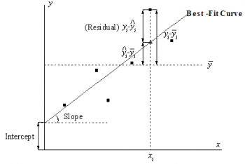
The figure below illustrates the concept to a simple linear model (Note that multiple regression and nonlinear fitting are similar).

Illustration of the Least Squares Method.png

The Best-Fit Curve represents the assumed theoretical model. For a particular point $(x_i,y_i)\,\!$ in the original dataset, the corresponding theoretical value at $x_i\,\!$ is denoted by $\widehat{y_i}$ .

If there are two independent variables in the regression model, the least square estimation will minimize the deviation of experimental data points to the best fitted surface. When there are more then 3 independent variables, the fitted model will be a hypersurface. In this case, the fitted surface (or curve) will not be plotted when regression is performed.

Origin provides two options to adjust the parameter values in the iterative procedure

Levenberg-Marquardt (L-M) Algorithm

The Levenberg-Marquardt (L-M) algorithm¹¹ is a iterative procedure which combines the Gauss-Newton method and the steepest descent method. The algorithm works well for most cases and become the standard of nonlinear least square routines.

Compute the $\chi ^2(b)$ value from the given initial values: $b$ .
Pick a modest value for $\lambda$ , say $\lambda$ = 0.001
Solve the Levenberg-Marquardt funciton¹¹ for $\delta b$ and evaluate $\chi ^2(\beta + \delta b)$
If $\chi ^2(\beta + \delta b) \geq \chi ^2(b)$ ,increase $\lambda$ by a factor of 10 and go back to step 3
if $\chi ^2(\beta + \delta b) \leq \chi ^2(b)$ , decrease $\lambda$ by a factor of 10, update the parameter values to be $\delta b$ and go back to step 3
Stop until the values computed in two successive iterations are small enough (compared with the tolerance)

Downhil Simplex Algorithm

Besides the L-M method, Origin also provides a Downhill Simplex approximation^9,10. In geometry, a simplex is a polytope of N + 1 vertices in N dimensions. In non-linear optimization, an analog exists for an objective function of N variables. During the iterations, the Simplex algorithm (also known as Nelder-Mead) adjusts the parameter "simplex" until it converges to a local minimum.

Different from L-M method, the Simplex method does not require derivatives, and it is effective when the computational burden is small. Normally, if you did not get a good value for parameter initialization, you can try this method to get the approximate parameter value for further fitting calculations with L-M. The Simplex method tends to be more stable in that it is less likely to wander into a meaningless part of the parameter space; on the other hand, it is generally much slower than L-M, especially very close to a local minimum. Actually, there is no "perfect" algorithm for nonlinear fitting, and many things may affect the result (e.g., initial values). In complicated models, you may find one method may do better than the other. Additionally, you may want to try both methods to perform the fitting operation.

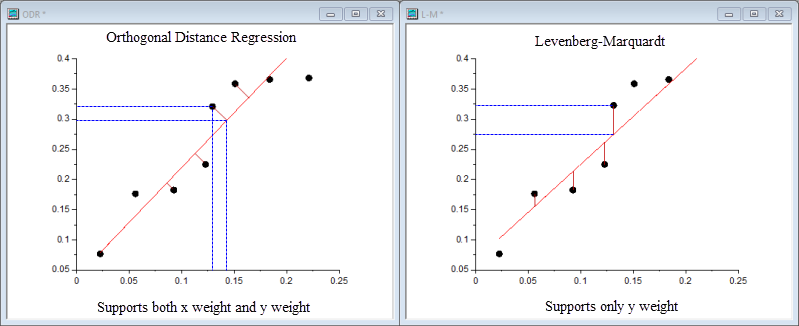
Orthogonal Distance Regression (ODR) Algorithm

The Orthogonal Distance Regression (ODR) algorithm minimizes the residual sum of squares by adjusting both fitting parameters and values of the independent variable in the iterative process. The residual in ODR is not the difference between the observed value and the predicted value for the dependent variable, but the orthogonal distance from the data to the fitted curve.

Origin uses the ODR algorithm in ODRPACK95⁸.

For a explict function, the ODR algorithm could be expressed as:

$\min\left (\sum_{i=1}^{n}\left (w_{yi}\cdot \epsilon_{i} ^{2}+w_{xi}\cdot \delta_{i}^{2} \right ) \right )$

subject to the constraints:

$y_{i}=f\left ( x_{i} +\delta_{i}; \beta \right )-\epsilon _{i}\ \ \ \ \ \ i=1,...,n$

where $w_{xi}$ and $w_{yi}$ are the user input weights of $x_{i}$ and $y_{i}$ , $\delta_{i}$ and $\epsilon_{i}$ are the residual of the corresponding $x_{i}$ and $y_{i}$ , and $\beta$ is the fitting parameter.

For more details of the ODR algorithm, please refer to ODRPACK95⁸.

Comparison between ODR and L-M

To choose the ODR or L-M algorithm for your fitting, you may refer to the following table for information:

	Orthogonal Distance Regression	Levenberg-Marquardt
Application	Both implicit and explicit functions	Only explicit functions
Weight	Support both x weight and y weight	Support only y weight
Residual Source	The orthogonal distance from the data to the fitted curve	The difference between the observed value and the predicted value
Iteration Process	Adjusting the values of fitting parameters and independent variables	Adjusting the values of fitting parameters

Implicit Functions

Fitting Model

A general implicit function could be expressed as:

$f\left ( X, Y, \beta \right )-const=0$

(5)

where $X = (x_1, x_2, \cdots , x_k)'$ and $Y = (y_1, y_2, \cdots , y_k)'$ are the variables, $\beta$ are the fitting parameters and $const$ is a constant.

Examples of the Implicit Function:

$f = \left(\frac{x-x_c}{a}\right)^2 + \left(\frac{y-y_c}{b}\right)^2 - 1$

Orthogonal Distance Regression (ODR) Algorithm

The ODR method can be used for both implicit functions and explicit functions. To learn more details of ODR method, please refer to the description of ODR mehtod in above section

For implicit functions, the ODR algorithm could be expressed as:

$\min\left (\sum_{i=1}^{n}\left ( w_{xi}\cdot \delta_{xi}^{2}+w_{yi}\cdot \delta_{yi}^{2} \right ) \right )$

subject to:

$f\left ( x_{i}+\delta_{xi},y_{i}+\delta_{yi},\beta \right )= 0\ \ \ \ \ \ i=1,...,n$

where $w_{xi}$ and $w_{yi}$ are the user input weights of $x_{i}$ and $y_{i}$ , $\delta_{xi}$ and $\delta_{yi}$ are the residual of the corresponding $x_{i}$ and $y_{i}$ , and $\beta$ is the fitting parameter.

Weighted Fitting

When the measurement errors are unknown, $\sigma _i\,\!$ are set to 1 for all i, and the curve fitting is performed without weighting. However, when the experimental errors are known, we can treat these errors as weights and use weighted fitting. In this case, the chi-square can be written as:

$\chi ^2=\sum_{i=1}^nw_i[Y_i-f(x_i^{\prime },\hat \beta )]^2$

(6)

There are a number of weighting methods available in Origin. Please read Fitting with Errors and Weighting in the Origin Help file for more details.

Parameters

The fit-related formulas are summarized here:

The Fitted Value

Computing the fitted values in nonlinear regression is an iterative procedure. You can read a brief introduction in the above section (How Origin Fits the Curve), or see the below-referenced material for more detailed information.

Parameter Standard Errors

During L-M iteration, we need to calculate the partial derivatives matrix F, whose element in ith row and jth column is:

$F_{ij}=\frac{\partial f(x,\theta )}{\sigma _i\partial \theta _j}$

(7)

where $\sigma _i$ is the error of y for the ith observation if Instrumental weight is used. If there is no weight, $\sigma _i = 1$ . And $F_{ij}$ is evaluated for each observation $x_i$ in each iteration.

Then we can get the Variance-Covariance Matrix for parameters by:

$C=(F'F)^{-1}s^2\,\!$

(8)

where $F'$ is the transpose of the F matrix, s² is the mean residual variance, also called Reduced Chi-Sqr, or the Deviation of the Model, and can be calculated as follows:

$s^2=\frac{RSS}{n-p}$

(9)

where n is the number of points, and p is the number of parameters.

The square root of the main diagonal value of this matrix C is the Standard Error of the corresponding parameter

$s_{\theta _i}=\sqrt{c_{ii}}\,\!$

(10)

where C_ii is the element in ith row and ith column of the matrix C. C_ij is the covariance between θ_i and θ_j.

You can choose whether to exclude s² when calculating the covariance matrix. This will affect the Standard Error values. When excluding s², clear the Use reduce Chi-Sqr check box on the Advanced page under Fit Control panel. The covariance is then calculated by:

$c=(F'F)^{-1}\,\!$

(11)

So the Standard Error now becomes:

$s_{\theta _i}^{\prime }=\frac{s_{\theta _i}}s\,\!$

(12)

The parameter standard errors can give us an idea of the precision of the fitted values. Typically, the magnitude of the standard error values should be lower than the fitted values. If the standard error values are much greater than the fitted values, the fitting model may be overparameterized.

The Standard Error for Derived Parameter

Origin estimates the standard errors for the derived parameters according to the Error Propagation formula, which is an approximate formula.

Let $z = f\left (\theta _1, \theta _2, ..., \theta _p \right )$ be the function with a combination (linear or non-linear) of $p\,$ variables $\theta _1, \theta _2, ..., \theta _p \,$ .

The general law of error propagation is:

$\sigma_z^2 = \sum_i^p \sum_j^p \frac {\partial z}{\partial \theta_i} COV_{\theta_i \theta_j} \frac {\partial z}{\partial \theta_j}$

where $COV_{\theta_i \theta_j}\,$ is the covariance value for $\left (\theta_i, \theta_j \right )$ , and $\left (i = 1, 2, ..., p \right ), \left (j = 1, 2, ..., p \right )$ .

You can choose whether to exclude mean residual variance $s^2$ when calculating the covariance matrix $COV_{\theta_i \theta_j}$ , which affects the Standard Error values for derived parameters. When excluding $s^2$ , clear the Use reduce Chi-Sqr check box on the Advanced page under Fit Control panel.

For example, using three variables

$z = f\left (\theta_1, \theta_2, \theta_3 \right )$

we get:

$\sigma_z^2 = \left (\frac {\partial z}{\partial \theta_1} \right )^2 \sigma_{\theta_1}^2 + \left (\frac {\partial z}{\partial \theta_2} \right )^2 \sigma_{\theta_2}^2 + \left (\frac {\partial z}{\partial \theta_3} \right )^2 \sigma_{\theta_3}^2 + 2 \left (\frac {\partial z}{\partial \theta_1} \frac {\partial z}{\partial \theta_2} \right ) COV_{\theta_1 \theta_2} + 2 \left (\frac {\partial z}{\partial \theta_1} \frac {\partial z}{\partial \theta_3} \right ) COV_{\theta_1 \theta_3} + 2 \left (\frac {\partial z}{\partial \theta_2} \frac {\partial z}{\partial \theta_3} \right ) COV_{\theta_2 \theta_3}$

Now, let the derived parameter be $z\,$ , and let the fitting parameters be $\theta_1, \theta_2, ..., \theta_p\,$ . The standard error for the derived parameter $z\,$ is $\sigma_z\,$ .

Confidence Intervals

Origin provides two methods to calculate the confidence intervals for parameters: Asymptotic-Symmetry method and Model-Comparison method.

Asymptotic-Symmetry Method

One assumption in regression analysis is that data is normally distributed, so we can use the standard error values to construct the Parameter Confidence Intervals. For a given significance level, α, the (1-α)x100% confidence interval for the parameter is:

$\hat \theta _j-t_{(\frac \alpha 2,n-p)}s_{\theta _j}\leq \hat \theta _j\leq \hat \theta _j+t_{(\frac \alpha 2,n-p)}s_{\theta _j}$

(13)

The parameter confidence interval indicates how likely the interval is to contain the true value.

The confidence interval illustrated above is Asymptotic, which is the most frequently used method to calculate the confidence interval. The "Asymptotic" here means it is an approximate value.

Model-Comparison Method

If you need more accurate values, you can use the Model Comparison Based method to estimate the confidence interval.

If the Model Comparison method is used, the upper and lower confidence limits will be calculated by searching for the values of each parameter p that makes RSS(θ_j) (minimized over the remaining parameters) greater than RSS by a factor of (1+F/(n-p)).

$RSS(\theta _j)=RSS(1+F\frac 1{n-p})$

(14)

where F = Ftable(α,1,n-p)and RSS is the minimum residual sum of square found during the fitting session.

t Value

You can choose to perform a t-test on each parameter to see whether its value is equal to 0. The null hypothesis of the t-test on the jth parameter is:

$H_0: \theta_j = 0 \,$

And the alternative hypothesis is:

$H_\alpha : \theta_j \ne 0$

The t-value can be computed as:

$t=\frac{\hat \beta _j-0}{s_{\hat \beta _j}}$

(15)

Prob>|t|

The probability that H₀ in the t test above is true.

$prob=2(1-tcdf(|t|,df_{Error}))\,\!$

(16)

where tcdf(t, df) computes the lower tail probability for Student's t distribution with df degree of freedom.

Dependency

If the equation is overparameterized, there will be mutual dependency between parameters. The dependency for the ith parameter is defined as:

$1-\frac 1{c_{ii}(c^{-1})_{ii}}$

(17)

and (C^-1)_ii is the (i, i)th diagonal element of the inverse of matrix C. If this value is close to 1, there is strong dependency.

To learn more about how the value assess the quality of a fit model, see Model Diagnosis Using Dependency Values page

CI Half Width

The Confidence Interval Half Width is:

$CI=\frac{UCL-LCL}2$

(18)

where UCL and LCL is the Upper Confidence Interval and Lower Confidence Interval, respectively.

Statistics

Several fit statistics formulas are summarized below:

Degree of Freedom

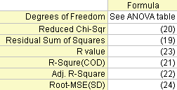
The Error degree of freedom. Please refer to the ANOVA Table for more details.

Residual Sum of Squares

The residual sum of squares:

$RSS(X,\hat \theta )=\sum_{i=1}^n w_i[Y_i-f(x_i^{\prime },\hat \theta )]^2$

(19)

Reduced Chi-Sqr

The Reduced Chi-square value, which equals the residual sum of square divided by the degree of freedom.

$Reduced\chi ^2=\frac{\chi ^2}{df_{Error}}=\frac{RSS}{df_{Error}}$

(20)

R-Square (COD)

The R² value shows the goodness of a fit, and can be computed by:

$R^2=\frac{Explained\,variation}{Total\,variation}=\frac{TSS-RSS}{TSS}=1-\frac{RSS}{TSS}$

(21)

where TSS is the total sum of square, and RSS is the residual sum of square.

Adj. R-Square

The adjusted R² value:

$\bar R^2=1-\frac{RSS/df_{Error}}{TSS/df_{Total}}$

(22)

R Value

The R value is the square root of R²:

$R=\sqrt{R^2}$

(23)

For more information on R², adjusted R² and R, please see Goodness of Fit.

Root-MSE (SD)

Root mean square of the error, or the Standard Deviation of the residuals, equal to the square root of reduced χ²:

$Root\,MSE=\sqrt{Reduced \,\chi ^2}$

(24)

ANOVA Table

The ANOVA Table:

Note: The ANOVA table is not available for implicit function fitting.

	df	Sum of Squares	Mean Square	F Value	Prob > F
Model	p	SS_reg = TSS - RSS	MS_reg = SS_reg / p	MS_reg / MSE	p-value
Error	n - p	RSS	MSE = RSS / (n - p)
Uncorrected Total	n	TSS
Corrected Total	n-1	TSS_corrected

Note: In nonlinear fitting, Origin outputs both corrected and uncorrected total sum of squares: Corrected model:

$TSS_{corrected}=\sum_{i=1}w_{i}y_{i}^2-\left(\sum_{i=1}\left(y_{i}w_{i} \right )/\sum_{i=1}w_{i} \right )^2\sum_{i=1}w_{i}$

(25)

Uncorrected model:

$TSS=\sum_{i=1}^nw_iy_i^2$

(26)

The F value here is a test of whether the fitting model differs significantly from the model y=constant. Additionally, the p-value, or significance level, is reported with an F-test. We can reject the null hypothesis if the p-value is less than $\alpha\,\!$ , which means that the fitting model differs significantly from the model y=constant.

Confidence and Prediction Bands

Confidence Band

The confidence interval for the fitting function says how good your estimate of the value of the fitting function is at particular values of the independent variables. You can claim with 100α% confidence that the correct value for the fitting function lies within the confidence interval, where α is the desired level of confidence. This defined confidence interval for the fitting function is computed as:

$f(x_{1i},x_{2i},\ldots ;\theta _{1i},\theta _{2i},\ldots )\pm t_{(\frac \alpha 2,dof)}[s^2fcf^{\prime }]^{\frac 12}$

(27)

where:

$f=[\frac{\partial f}{\partial \theta _1},\frac{\partial f}{\partial \theta _2},\cdots ,\frac{\partial f}{\partial \theta _p}]$

(28)

Prediction Band

The prediction interval for the desired confidence level α is the interval within which 100α% of all the experimental points in a series of repeated measurements are expected to fall at particular values of the independent variables. This defined prediction interval for the fitting function is computed as:

$f(x_{1i},x_{2i},\ldots ;\theta _{1i},\theta _{2i},\ldots )\pm t_{(\frac \alpha 2,dof)}[s^2(1+fcf^{\prime })]^{\frac 12}$

(29)

where

$\chi _*^2$ is Reduced $\chi ^2$

Notes: The Confidence Band and Prediction Band in the fitted curve plot are not available for implicit function fitting.

Topics for Further Reading

Reference

William. H. Press, etc. Numerical Recipes in C++. Cambridge University Press, 2002.
Norman R. Draper, Harry Smith. Applied Regression Analysis, Third Edition. John Wiley & Sons, Inc. 1998.
George Casella, et al. Applied Regression Analysis: A Research Tool, Second Edition. Springer-Verlag New York, Inc. 1998.
G. A. F. Seber, C. J. Wild. Nonlinear Regression. John Wiley & Sons, Inc. 2003.
David A. Ratkowsky. Handbook of Nonlinear Regression Models. Marcel Dekker, Inc. 1990.
Douglas M. Bates, Donald G. Watts. Nonlinear Regression Analysis & Its Applications. John Wiley & Sons, Inc. 1988.
Marko Ledvij. Curve Fitting Made Easy. The Industrial Physicist. Apr./May 2003. 9:24-27.
"J. W. Zwolak, P.T. Boggs, and L.T. Watson, ``Algorithm 869: ODRPACK95: A weighted orthogonal distance regression code with bound constraints, ACM Transactions on Mathematical Software Vol. 33, Issue 4, August 2007."
Nelder, J.A., and R. Mead. 1965. Computer Journal, vol. 7, pp. 308 -313
Numerical Recipes in C, Ch. 10.4, Downhill Simplex Method in Multidimensions.
Numerical Recipes in C, Ch. 15.5, Nonlinear Models.

15.3.3 Theory of Nonlinear Curve Fitting

Contents

How Origin Fits the Curve

Explicit Functions

Fitting Model

Least-Squares Algorithms

Levenberg-Marquardt (L-M) Algorithm

Downhil Simplex Algorithm

Orthogonal Distance Regression (ODR) Algorithm

Comparison between ODR and L-M

Implicit Functions

Fitting Model

Orthogonal Distance Regression (ODR) Algorithm

Weighted Fitting

Parameters

The Fitted Value

Parameter Standard Errors

The Standard Error for Derived Parameter

Confidence Intervals

Asymptotic-Symmetry Method

Model-Comparison Method

t Value

Prob>|t|

Dependency

CI Half Width

Statistics

Degree of Freedom

Residual Sum of Squares

Reduced Chi-Sqr

R-Square (COD)

Adj. R-Square

R Value

Root-MSE (SD)

ANOVA Table

Confidence and Prediction Bands

Confidence Band

Prediction Band

Topics for Further Reading

Reference